I gave a talk at the Hong Kong Machine Learning Meetup on 17th April 2019. These are the slides from that talk.
Category: Neural Networks
The SQuAD Challenge – Machine Comprehension on the Stanford Question Answering Dataset
The SQuAD Challenge
Machine Comprehension on the
Stanford Question Answering Dataset
Over the past few years have seen some significant advances in NLP tasks like Named Entity Recognition [1], Part of Speech Tagging [2] and Sentiment Analysis [3]. Deep learning architectures have replaced conventional Machine Learning approaches with impressive results. However, reading comprehension remains a challenging task for machine learning [4][5]. The system has to be able to model complex interactions between the paragraph and question. Only recently have we seen models come close to human level accuracy (based on certain metrics for a specific, constrained task). For this paper I implemented the Bidirectional Attention Flow model [6], using pretrained word vectors and training my own character level embeddings. Both these were combined and passed through multiple deep learning layers to generated a query aware context representation of the paragraph text. My model achieved 76.553% F1 and 66.401% EM on the test set.
Introduction
2014 saw some of the first scientific papers on using neural networks for machine translation (Bahdanau, et al [7], Kyunghyun et al [8], Sutskever, et al [9]). Since then we have seen an explosion in research leading to advances in Sequence to Sequence models, multilingual neural machine translation, text summarization and sequence labeling.
Machine comprehension evaluates a machine’s understanding by posing a series of reading comprehension questions and associated text, where the answer to each question can be found only in its associated text [5]. Machine comprehension has been a difficult problem to solve – a paragraph would typically contain multiple sentences and Recurrent Neural Networks are known to have problems with long term dependencies. Even though LSTMs and GRUs address the exploding/vanishing gradients RNNs experience, they too struggle in practice. Using just the last hidden state to make predictions means that the final hidden state must encode all the information about a long word sequence. Another problem has been the lack of large datasets that deep learning models need in order to show their potential. MCTest [10] has 500 paragraphs and only 2,000 questions.
Rajpurkar, et al addressed the data issue by creating the SQuAD dataset in 2016 [11]. SQuAD uses articles sourced from Wikipedia and has more than 100,000 questions. The labelled data was obtained by crowdsourcing on Amazon Mechanical Turk – three human responses were taken for each answer and the official evaluation takes the maximum F1 and EM scores for each one.
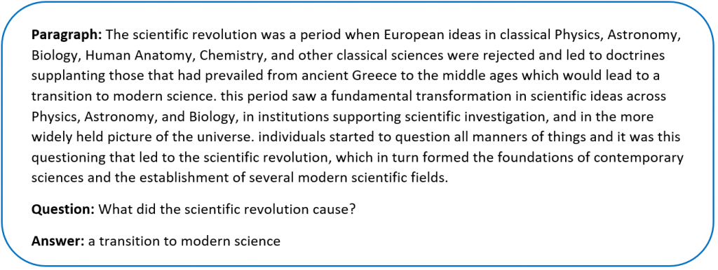
Sample SQuAD dataSince the release of SQuAD new research has pushed the boundaries of machine comprehension systems. Most of these use some form of Attention Mechanism [6][12][13] which tell the decoder layer to “attend” to specific parts of the source sentence at each step. Attention mechanisms address the problem of trying to encode the entire sequence into a final hidden state.
Formally we can define the task as follows – given a context paragraph c, a question q we need to predict the answer span by predicting (astart,aend) which are start and end indices of the context text where the answer lies.
For this project I implemented the Bidirectional Attention Flow model [6] – a hierarchical multi-stage model that has performed very well on the SQuAD dataset. I trained my own character vectors [15][16], and used pretrained Glove embeddings [14] for the word vectors. My final submission was a single model – ensemble models would typically yield better results but the complexity of my model meant longer training times.
Related Work
Since its introduction in June 2016, the SQuAD dataset has seen lots of research teams working on the challenge. There is a leaderboard maintained at https://rajpurkar.github.io/SQuAD-explorer/. Submissions since Jan 2018 have beaten human accuracy on one of the metrics (Microsoft Research, Alibaba and Google Brain are on this list at the time of writing this paper). Most of these models use some form of attention mechanism and ensemble multiple models.
For example, the R-Net by Microsoft Research [12] is a high performing SQuAD model. They use word and character embeddings along with Self-Matching attention. The Dynamic Coattention Network [13], another high performing SQuAD model uses coattention.
Approach
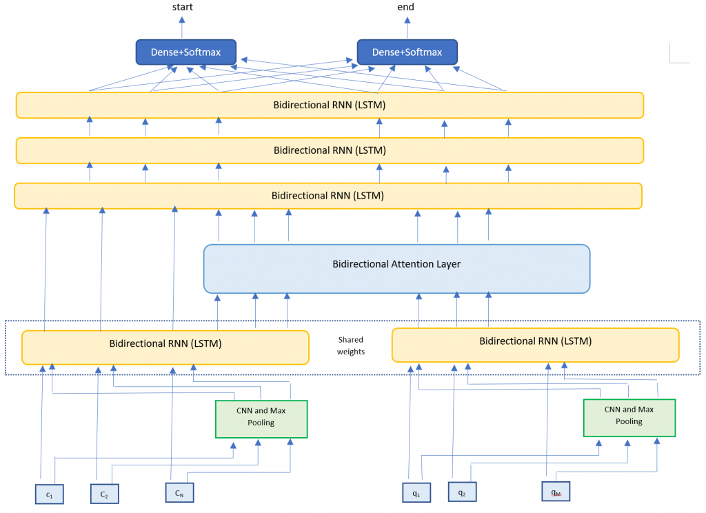
My model architecture is very closely based on the BiDAF model [6]. I implemented the following layers
- Embedding layer – Maps words to high dimensional vectors. The embedding layer is applied separately to both the context and question text. I used two methods
- Word embeddings – Maps each word to pretrained vectors. I used 300 dimensional GloVE vectors.
- Character embeddings – Maps each word to character embedding and run them through multiple layers of Convolutions and Max Pooling layers. I trained my own character embeddings due to challenges with the dataset.
- RNN Encoder layer – Takes the context and question embeddings and runs each one through a Bi-Directional RNN (LSTM). The Bi-RNNs share weights in order to enrich the context-question relationship.
- Attention Layer – Calculates the BiDirectional attention flow (Context to Query attention and Query to Context attention). We concatenate this with the context embeddings.
- Modeling Layer – Runs the attention and context layers through multiple layers of Bi-Directional RNNs (LSTMs)
- Output layer – Runs the output of the Modeling Layer through two fully connected layers to calculate the start and end indices of the answer span.
Dataset
The dataset for this project was SQuAD – a reading comprehension dataset. SQuAD uses articles sourced from Wikipedia and has more than 100,000 questions. Our task is to find the answer span within the paragraph text that answers the questions.
The sentences (all converted to lowercase) are tokenized into words using nltk. The words are then converted into high dimensional vector embeddings using Glove. The characters for each word are also converted into character embeddings and then run through a series of convolutions neural network and max pooling layers. I ran some analysis on the word and character counts in the dataset to better understand what model parameters to use.
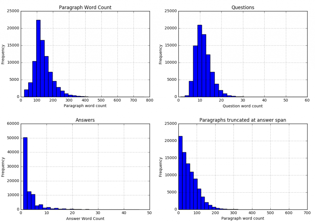 We can see that
| 99.8 percent of paragraphs are under 400 words |
| 99.9 percent of questions are under 30 words |
| 99 percent of answers are under 20 words (97.6 under 15 words) |
| 99.9 percent of answer spans lie within first 300 paragraph words |
We can use these statistics to adjust our model parameters (described in the next section).
For the character level encodings, I did an analysis of the character vocabulary in the training text. We had 1,258 unique characters. Since we are using Wikipedia for our training set, many articles contain foreign characters.

Further analysis suggested that these special characters don’t really affect the meaning of a sentence for our task, and that the answer span contained 67 unique characters. I therefore selected these 67 as my character vocabulary and replaced all the others with a special REPLACEMENT TOKEN.
Instead of using one-hot embeddings for character vectors, I trained my own character vectors on a subset of Wikipedia. I ran the word2vec algorithm at a character level to get char2vec 50 dimensional character embeddings. A t-SNE plot of the embeddings shows us results similar to word2vec.
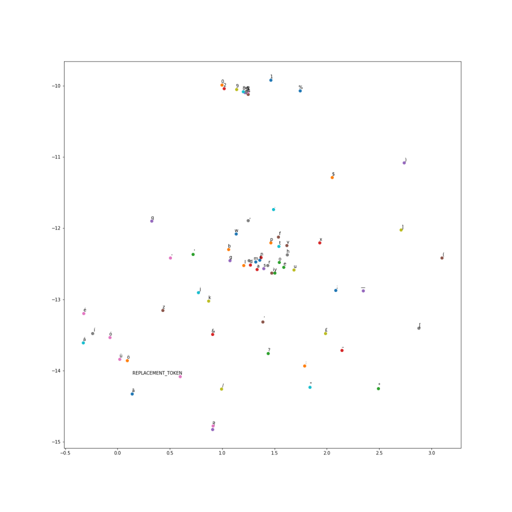 I used these trained character vectors for my character embeddings. The maximum length of a paragraph word was 37 characters, and 30 characters for a question word. Since we are using max pooling, I used these as my character dimensions and padded with zero vectors for smaller words.
Model Configuration
I used the following parameters for my model. Some of these (context length, question length, etc.) were fixed based on the data analysis in the previous section. Others were set by trying different parameters to see which ones gave the best results.
| Parameter | Description | Value |
| context_len | Number of words in the paragraph input | 300 |
| question_len | Number of words in the question input | 30 |
| embedding_size | Dimension of GLoVE embeddings | 300 |
| context_char_len | Number of characters in each word for the paragraph input (zero padded) | 37 |
| question_char_len | Number of characters in each word for the question input (zero padded) | 30 |
| char_embed_size | Dimension of character embeddings | 50 |
| optimizer | Optimizer used | Adam |
| learning_rate | Learning Rate | 0.001 |
| dropout | Dropout (used one dropout rate across the network) | 0.15 |
| hidden_size | Size of hidden state vector in the Bi-Directional RNN layers | 200 |
| conv_channel_size | Number of channels in the Convolutional Neural Network | 128 |
Evaluation metric
Performance on SQuAD was measured via two metrics:
- ExactMatch (EM) – Binary measure of whether the system output matches the ground truth exactly.
- F1 – Harmonic mean of precision and recall.
Results
My model achieved the following results (I scored much higher on the Dev and Test leaderboards than on my Validation set)
| Dataset | F1 | EM |
| Train | 81.600 | 68.000 |
| Val | 69.820 | 54.930 |
| Dev | 75.509 | 65.497 |
| Test | 76.553 | 66.401 |
The original BiDAF paper had an F1 score of 77.323 and EM score of 67.947. My model scored a little lower, possibly because I am missing some details not mentioned in their paper, or I need to tweak my hyperparameters further. Also, my scores were lower running against my cross validation set vs the official competition leaderboard.
I tracked accuracy on the validation set as I added more complexity to my model. I found it interesting to understand how each additional element contributed to the overall score. Each row tracks the added complexity and scores related to adding that component.
| Model | F1 | EM |
| Baseline | 39.34 | 28.41 |
| BiDAF | 42.28 | 31.00 |
| Smart Span (adjust answer end location) | 44.61 | 31.13 |
| 1 Bi-directional RNN in Modeling Layer | 66.83 | 51.40 |
| 2 Bi-directional RNNs in Modeling Layer | 68.28 | 53.10 |
| 3 Bi-directional RNNs in Modeling Layer | 68.54 | 53.25 |
| Character CNN | 69.82 | 54.93 |
I also analyzed the questions where we scored zero on F1 and EM scores. The F1 score is more forgiving. We would have a non zero F1 if we predict even one word correctly vs any of the human responses. An analysis of questions that scored zero on the F1and EM metric were split by question type. The error rates are proportional to the distribution of the questions in the dataset.
| Question Type | Entire Dev Set (%) | F1=0 (%) | EM=0 (%) |
| what | 27.2 | 28.4 | 29.3 |
| is | 18.4 | 18.5 | 18.4 |
| did | 9.1 | 8.8 | 9.0 |
| was | 8.7 | 9.1 | 7.9 |
| do | 6.9 | 6.9 | 7.9 |
| how | 6.2 | 5.9 | 6.1 |
| who | 6.2 | 6.7 | 6.1 |
| are | 4.4 | 3.7 | 4.2 |
| which | 3.3 | 3.4 | 3.1 |
| where | 2.3 | 2.5 | 2.5 |
| when | 3.9 | 2.9 | 2.3 |
| name | 1.8 | 1.5 | 1.5 |
| why | 0.7 | 0.6 | 1.3 |
| would | 0.7 | 0.9 | 0.9 |
| whose | 0.2 | 0.2 | 0.2 |
However, there were some questions where the system was very close to the correct answer, or the correct answer was technically wrong
Conclusion
Attention mechanisms coupled with deep neural networks can achieve competitive results on Machine Comprehension. For this project I implemented the BiDirectional attention flow model. My model accuracy was very close to the original paper. In the modeling layer we discovered that deeper networks do increase accuracy, but at a steeper computational cost.
For future work I would like to explore an ensemble of models – using different deep learning layers and attention mechanisms. Looking at the leaderboard (https://rajpurkar.github.io/SQuAD-explorer/), most of the top performing models are ensembles.
Sentiment Analysis of movie reviews part 2 (Convolutional Neural Networks)
In a previous post I looked at sentiment analysis of movie reviews using a Deep Neural Network. That involved using pretrained vectors (GLOVE in our case) as a bag of words and fine tuning them for our task.
We will try a different approach to the same problem – using Convolutional Neural Networks (aka Deep Learning). We will take the idea from the image recognition blog and apply it to text classification. The idea is to
- Vectorize at a character level, using just the characters in our text. We don’t use any pretrained vectors for word embeddings.
- Apply multiple convolutional and max pooling layers to the data.
- Generate a final output layer with softmax
- We’re assuming the Convolutional Neural Network will automatically detect the relationship between characters (pooling them into words and further understanding the relationships between words).
Our input data is just vectorizing each character. We take all the unique characters in our data, and the maximum sentence length and transform our input data into maximum_sentence_length X character_count for each sentence. For sentences with less than the maximum_length, we pad the remaining rows with zeros.
I used 2 1-Dimensional convolutional layers with filter size=3, stride=1 and hidden size=64 and relu for the non-linear activation (see the Image Recognition blog for an explanation on this). I also added a pooling layer of size 3 after each convolution.
Finally, I used 2 fully connected layers of sizes 1024 and 256 dropout probability of 0.5 (that should help prevent over fitting. The final layer uses a softmax to generate the output probabilities and we the standard cross entropy function for the loss. The learning is optimized using the Adam optimizer.
Overall the results are very close to the deep neural network. We get 59.2% using CNNs vs 62%. I think the accuracy is the maximum information we can extract from this data. What’s interesting is we used 2 completely different approaches – pretrained word vectors in the Neural Network case, and character level vectors in this Deep Learning case and we got similar results.
Next post we will explore using LSTMs on the same problem.
Source code available on request.
Evaluation of Machine Learning Trading Strategies Using Recurrent Reinforcement Learning
A few months ago I did the Stanford CS221 course (Introduction to AI). The course was intense, covering a lot of advanced material. For the final project I worked with 2 teammates (Tesa Ho and Albert Lau) on evaluating Machine Learning Strategies using Recurrent Reinforcement Learning. This is our final project submission.
Introduction
There have been several studies that propose using Recurrent Reinforcement Learning to
design profitable trading systems over longer time horizons [see Moody , David and Molina ].
A common practice at trading shops today is to develop a Supervised Learning classification
algorithm to predict whether or not there will be a move of +/- X bps in the next t time period.
Depending on the trading strategy, the model selection may be based on maximizing the
Precision, Accuracy, a mixture of both i.e. F-score, or a measure of profit (i.e. Sharpe Ratio). In
the case of the latter, the parameters of the trading strategy must also be optimized which often
requires brute force.
The direct reinforcement approach, on the other hand, differs from dynamic programming and
reinforcement algorithms such as TD-learning and Q-learning, which attempt to estimate a value
function for the control problem. For finance in particular, the presence of large amounts noise
and non stationarity in the datasets can cause severe problems for the value function approach.
The RRL direct reinforcement framework enables a simpler problem representation, avoids
Bellman’s curse of dimensionality and offers compelling advantages in efficiency.
This project will apply the Recurrent Reinforcement Learning methodology to intraday trading on
the Hong Kong futures exchange specifically the Hang Seng futures. A gradient ascent of the
Sortino Ratio (or Downside Deviation Ratio) was used to calculate the optimized weights to
determine the trade signal. The results indicate that profitability is dependent on the maximum
position allowed (the variable μ). We also develop a trading strategy using the Reinforcement
Learning framework to adapt predictions from a Supervised Learning algorithm and compare
the results to the Recurrent Reinforcement Learning results.
Model and Approach
Our model is based on the work of Molina and Moody. We use Recurrent Reinforcement
Learning to maximize the Sharpe Ratio or Sortino Ratio for a financial asset (Hang Seng
Futures in our case) over a selected training period, then apply the optimized weight parameter
to a test period. The trades and profitability are saved and the process of training and testing is
repeated for all data.
This report is based on 5 minute open, high, low, close prices for the Hang Seng front-month
futures from November 1, 2016 to August 31, 2017. The close price was used as the price
array, px , and was the basis of the log normal returns, rt .
![]()
Other variables used in the model are:
M = the window size of returns used in the recurrent reinforcement learning
N = number of iterations for the RL algo
μ = max position size
δ = transaction costs in bps per trade
numTrainDays = the number of training days used
numTestDays = the number of test days used
The trader is assumed to take only long, neutral, or short positions with a maximum position of
magnitude mu. The position Ft is established or maintained at the end of each time interval t
and is reassessed at the end of period t+1. Where Moody used a trader function of:
![]()
We opt to use a risk adjusted trader function of:
![]()
where
![]()
The trade cost, δ , associated with each trade is assumed to occur on the closing price at the
end of each time period t. A non-zero trading cost in bps is used to account for slippage, bid
ask spread, and associated trading fees.
The trade return, Rt , is defined as the return obtained from trading:
![]()
where
μ = maximum number of shares per transaction
δ = transaction cost in bps
The reward function that is traditionally used to compare trading strategies is the Sharpe Ratio.
The Sharpe Ratio takes the average of the trade returns divided by the standard deviation of the
trade returns. This penalizes strategies with large variance in returns.
![]()
However, variance in positive returns is acceptable so the Sortino Ratio, or Downside Deviation
Ratio, is a much more accurate measure of a strategy. The Sortino Ratio penalizes large
variations in negative.
![]()
The reinforcement learning algorithm adjusts the parameters of the system to maximize the
expected reward function. It can also be expressed as a function of profit or wealth, U(WT) , or
in our case, a function of the sequence of trading returns, U(R1 , R2 , …, RT). Given the trading
system Ft(θ) , we can then adjust the parameters θ to maximize UT . The optimized variable is
θ , an array of weights applied to the log normal price returns r_t−M , …, rt .
![]()
The gradient with respect to θ is:
![Rendered by QuickLaTeX.com \[\frac{d U_T(\theta)}{d \theta} =\sum_{t=1}^T \frac{d U_t}{dR_t} \{ \frac{dR_t}{dF_t} \frac{dF_1}{d \theta} + \frac{d R_t}{d F_{t-1}} \frac{dF_{t-1}}{d \theta} \} \]](http://rohitapte.com/wp-content/ql-cache/quicklatex.com-52d8d732746b1e2065c055bc1e40d0d5_l3.png)
where
![]()
![]()
![]()
![Rendered by QuickLaTeX.com \[\frac{dU_t}{dR_t}=\frac{(Avg R_t^2-Avg R_t)R_t}{\sqrt{\frac{T}{T-1}} (Avg R_t^2-Avg(R_t)^2)^1.5} \]](http://rohitapte.com/wp-content/ql-cache/quicklatex.com-8ed057ffb04f8050e648defec31b350c_l3.png)
We can then maximize the Sharpe Ratio using Gradient Ascent or Stochastic Gradient Ascent to find the optimal weights for θ .
![]()
where
η = learning rate
Training and Testing Procedure
The overall algorithm utilized a rolling training and test period of 30 and 10 days.
- Training period 1-30 days, test period 30-40 days
- Run recurrent learning algorithm to maximize the Sortino Ratio by optimizing θ over the training period
- Apply the optimized θ to the test period and evaluate the trades and pnl
- Update the training period to 10-40 days, test period 40-50 days and repeat the process
Overall analysis was run over all the test periods with the positions and trades priced at the closing price for each time period, t. Cumulative pnl was used to evaluate the trading strategies rather than than returns since geometric cumulative returns were skewed by negative and close to zero return periods.
Evaluation and Error Analysis
For the base case we have extracted features using the market data (order book depth, cancellations, trades, etc.) and run a random forest algorithm to classify +/- 10 point moves in the future over 60 second horizons. Probabilities were generated for -1, 0, +1 classes and the largest probability determined the predicted class. The predicted signal of -1, 0, +1 was then passed to the recurrent reinforcement algorithm to determine what the risk adjusted pnl would be.
For the oracle, we pass the actual target signals to the recurrent reinforcement learning algorithm to see what the maximum trading pnl would be.
We want to see if the recurrent reinforcement learning algorithm can generate better results.
We will additionally explore if we can use LSTMs to predict the next price and see if they perform better than our base case. We will also explore adding the predicted log return into our Reinforcement learning model as an additional parameter to compare results.
1. Oracle
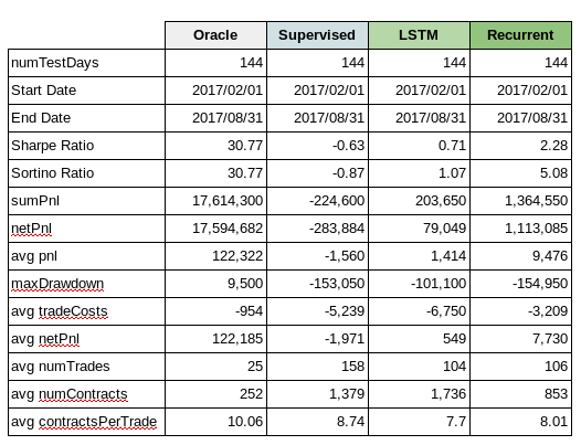
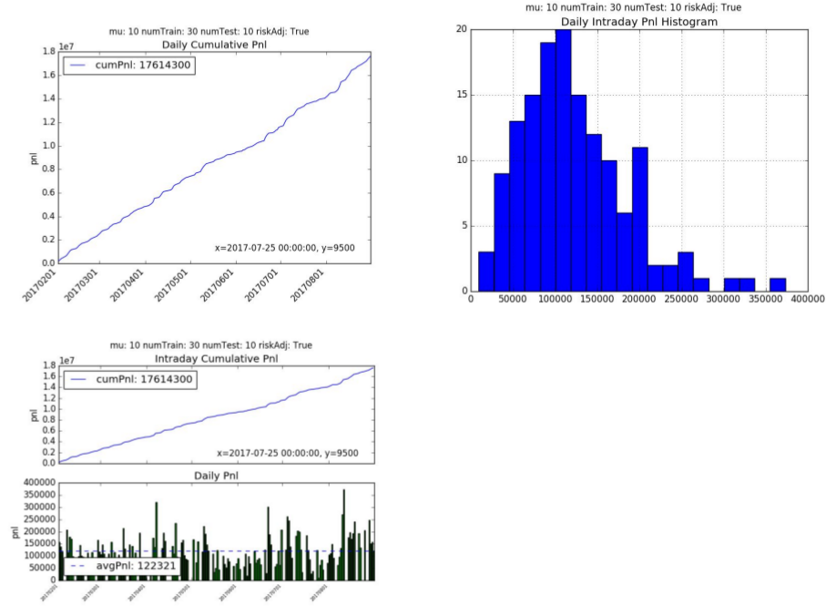
The Oracle cumulative pnl over a 144 day test period is 17.6mm hkd. The average daily pnl is 122,321 hkd per day. The annualized Sharpe and Sortino ratio is 30.77 with an average of 25 trades a day.
2. Recurrent Reinforcement Learning
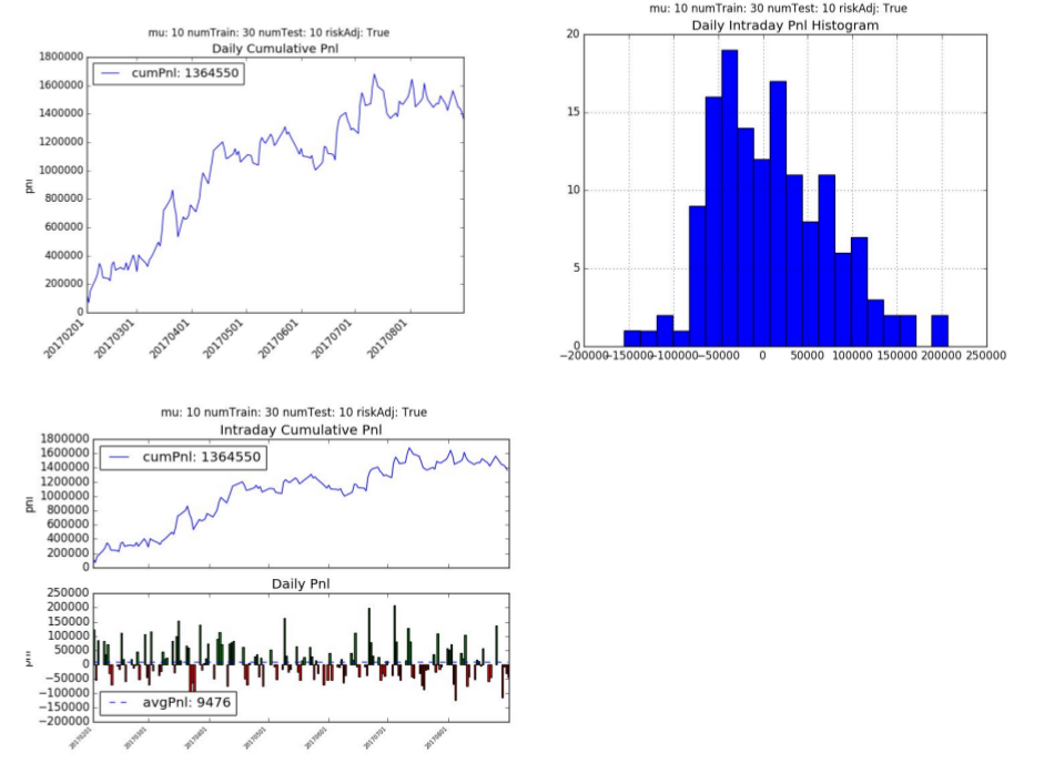
The recurrent reinforcement learning cumulative pnl is 1.35 mm hkd with an average daily pnl is 9,476 hkd per day. The annualized Sharpe Ratio is 2.28 and Sortino Ratio is 5.08. The average number of trades per day is 106 with 8 contracts per trade.
3. Supervised Learning
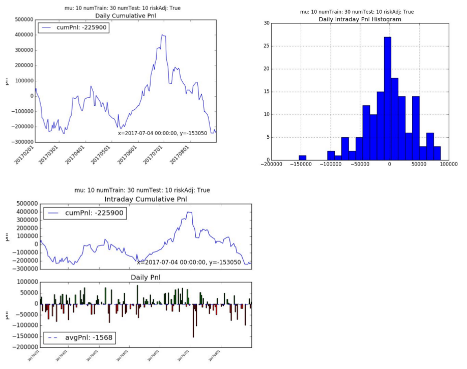
The supervised learning cumulative pnl is -226k hkd with an average daily pnl is -1568 hkd per day. The supervised learning model did not fair well with this trading strategy and had a Sharpe Ratio of -0.63 and Sortino Ratio of -0.87. The supervised learning algorithm traded much more frequently on average of 1,379 times a day with an average of 8.74 contracts per trade.
4. LSTM for Prediction
We also explored using LSTMs to predict +/- 10 point moves in the future over 60 second horizons. We used 30 consecutive price points (i.e. 30 minutes of trading data) to generate probabilities for (-1, 0 and +1).
One of the challenges we faced is the dataset is highly unbalanced, with approximately 94% of the cases being 0 (i.e. less than 10-tick move) and just 3% of the cases each being -1 (-10 tick move) or +1 (+10 tick move). Initially the LSTM was just calculating all items as 0 and getting a low error rate. We had to adjust our cross_entropy function to factor in the weights of the distribution which forced it try and classify the -1 and +1 more correctly.
We used a 1 layer LSTM with 64 hidden cells and a dropout of 0.2. Over the results were not great, but slightly better than the RandomForest.
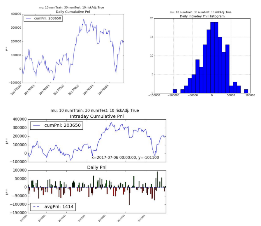
The cumulative pnl is +203.65k hkd with an average daily pnl is +1414 hkd per day. The model had a Sharpe Ratio of 0.71 and Sortino Ratio of 1.07. The algorithm traded less frequently than supervised learning (on average of 104 times a day) but traded larger contracts. This makes sense since it’s classifying only a small percentage of the +/- 1 correctly.
5. Variable Sensitivity Analysis
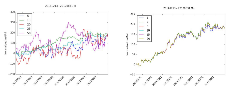
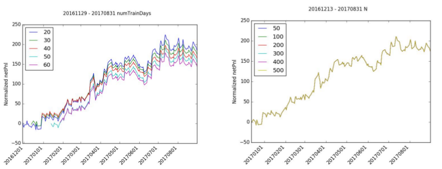
A sensitivity analysis was run to the following variables: M, μ, numTrainingDays, and N.
The selection of the right window period, M, is very important to the accumulation of netPnl. While almost all of the normalized netPnl ends at the same value, M=10 is the only value that has a stable increasing netPnl. M=20 and M=5 all have negative periods and M=50 has a significant amount of variance.
There is relatively little effect in normalized netPnl by adjusting mu. mu=1 has a slight drop in normalized pnl but still follows the same path as the other iterations.
The number of training days has a limited effect on normalized netPnl since the shape of the pnl is roughly the same for each simulation. The starting point difference indicates that the starting month may or may not have been good months for trading. In particular, trading in January 2017 looked to be positive while the month of December was slightly negative.
Likewise, the number of iterations, N, has very little effect on normalized netPnl. The normalized netPnl is virtually identical for all levels of N.
Conclusions
Recurrent Reinforcement Learning (RRL) shows promise in trading financial markets. While it lacks behind the oracle, this has significant improvements over the current business standards with the use of supervised learning. While the RRL approach is sensitive to the choice the window size, it is plausible to note its limited business adoption to-date possibly for the below reasons.
- We have tested the algorithms on 144 days of data. We need to validate the test on a
larger set of historical data. - Trade price assumption is based on closing price and not next period open price. In live markets there would be some slippage from the time a signal was generated to when a trade was executed.
- We assume our execution costs are static. For larger trades, there would be more
slippage. We are also not making any assumptions about trading margin, both for new trades and drawdowns. In live trading these factors would affect position sizing and trades. - Incorporation of supervised prediction did not include positional risk adjustment
Gradient calculation for Sortino Ratio - Since 2008 markets have largely been in a low volatility regime. We need to test this algorithm under stressed markets to ensure it performs as expected and that drawdowns are reasonable.
- In the past 12 months the market has seen some strong directional themes. A simple quantitative momentum strategy would likely yield similar results.
- Further work has to be done to determine if RRL algorithms can outperform well established quantitative strategies.
Sentiment Analysis of movie reviews part 1 (Neural Network)
I’ve always been fascinated with Natural Language Processing and finally have a few tools under my belt to tackle this in a meaningful way. There is an old competition on Kaggle for sentiment analysis on movie reviews. The link to the competition can be found here.
As per the Kaggle website – the dataset consists of tab-separated files with phrases from Rotten Tomatoes. Each sentence has been parsed into many phrases by the Stanford parser. Our job is to learn on the test data and make a submission on the test data. This is what the data looks like.
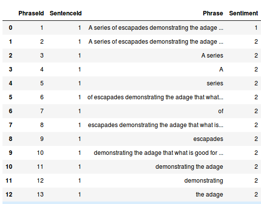
Each review (Sentiment in the above image) can take on values of 0 (negative), 1 (somewhat negative), 2 (neutral), 3 (somewhat positive) and 4 (positive). Our task is to predict the review based on the review text.
I decided to try a few techniques. This post will cover using a vanilla Neural Network but there is some work with the preprocessing of the data that actually gives decent results. In a future post I will explore more complex tools like LSTMs and GRUs.
Preprocessing the data is key here. As a first step we tokenized each sentence into words and vectorized the word using word embeddings. I used the Stanford GLOVE vectors. I assume word2vec would give similar results but GLOVE is supposedly superior since it captures more information of the relationships between words. Initially I ran my tests using the 50 dimensional vectors which gave about 60% accuracy on the test set and 57.7% on Kaggle. Each word then becomes a 50-dimensional vector.
For a sentence, we take the average of the word vectors as inputs to our Neural Network. This approach has 2 issues
- Some words don’t exist in the Glove database. We are ignoring them for now, but it may be useful to find some way to address this issue.
- Averaging the word embeddings means we fail to capture the position of the word in the sentence. That can have an impact on some reviews. For example if we had the following review
Great plot, would have been entertaining if not for the horrible acting and directing.
This would be a bad review but by averaging the word vectors we may be losing this information.
For the neural network I used 2 hidden layers with 1024 and 512 neurons. The final output goes through a softmax layer and we use the standard cross-entropy loss since this is a classification problem.
Overall the results are quite good. Using 100 dimensional GLOVE vectors, we get 62% accuracy on the test set and 60.8% on the Kaggle website.

Pre-trained vectors seem to be a good starting point to tackling NLP problems like this. The hyperparameter weight matrices will automatically tweak them for the task at hand.
Next steps are to explore larger embedding vectors and deeper neural networks to see if the accuracy improves further. Also play with regularization, dropout, and try different activation functions.
The next post will explore using more sophisticated techniques like LSTMs and GRUs.
Source code below (assuming you get the data from Kaggle)
|
1 2 3 4 5 6 7 8 9 10 11 12 13 14 15 16 17 18 19 20 21 22 23 24 25 26 27 28 29 30 31 32 33 34 35 36 37 38 39 40 41 42 43 44 45 46 47 48 49 50 51 52 53 54 55 56 57 58 59 60 61 62 63 64 |
import numpy as np import pandas as pd import numpy as np import csv #from nltk.tokenize import sent_tokenize,word_tokenize from nltk.tokenize import RegexpTokenizer from sklearn.preprocessing import LabelBinarizer from sklearn.model_selection import train_test_split glove_file='../glove/glove.6B.100d.txt' pretrained_vectors=pd.read_table(glove_file, sep=" ", index_col=0, header=None, quoting=csv.QUOTE_NONE) base_vector=pretrained_vectors.loc['this'].as_matrix() def vec(w): try: location=pretrained_vectors.loc[w] return location.as_matrix() except KeyError: return None def get_average_vector(review): numwords=0.0001 average=np.zeros(base_vector.shape) tokenizer = RegexpTokenizer(r'\w+') for word in tokenizer.tokenize(review): #sentences=sent_tokenize(review) #for sentence in sentences: # for word in word_tokenize(sentence): value=vec(word.lower()) if value is not None: average+=value numwords+=1 #else: # print("cant find "+word) average/=numwords return average.tolist() class SentimentDataObject(object): def __init__(self,test_ratio=0.1): self.df_train_input=pd.read_csv('/home/rohitapte/Documents/movie_sentiment/data/train.tsv',sep='\t') self.df_test_input=pd.read_csv('/home/rohitapte/Documents/movie_sentiment/data/test.tsv',sep='\t') self.df_train_input['Vectorized_review']=self.df_train_input['Phrase'].apply(lambda x:get_average_vector(x)) self.df_test_input['Vectorized_review'] = self.df_test_input['Phrase'].apply(lambda x: get_average_vector(x)) self.train_data=np.array(self.df_train_input['Vectorized_review'].tolist()) self.test_data=np.array(self.df_test_input['Vectorized_review'].tolist()) train_labels=self.df_train_input['Sentiment'].tolist() unique_labels=list(set(train_labels)) self.lb=LabelBinarizer() self.lb.fit(unique_labels) self.y_data=self.lb.transform(train_labels) self.X_train,self.X_cv,self.y_train,self.y_cv=train_test_split(self.train_data,self.y_data,test_size=test_ratio) def generate_one_epoch_for_neural(self,batch_size=100): num_batches=int(self.X_train.shape[0])//batch_size if batch_size*num_batches<self.X_train.shape[0]: num_batches+=1 perm=np.arange(self.X_train.shape[0]) np.random.shuffle(perm) self.X_train=self.X_train[perm] self.y_train=self.y_train[perm] for j in range(num_batches): batch_X=self.X_train[j*batch_size:(j+1)*batch_size] batch_y=self.y_train[j*batch_size:(j+1)*batch_size] yield batch_X,batch_y |
|
1 2 3 4 5 6 7 8 9 10 11 12 13 14 15 16 17 18 19 20 21 22 23 24 25 26 27 28 29 30 31 32 33 34 35 36 37 38 39 40 41 42 43 44 45 46 47 48 49 50 51 52 53 54 55 56 57 58 59 60 61 62 63 64 65 66 67 68 69 70 71 72 73 74 75 76 77 78 79 80 81 82 83 84 85 86 87 |
import tensorflow as tf import SentimentData #import numpy as np import pandas as pd sentimentData=SentimentData.SentimentDataObject() INPUT_VECTOR_SIZE=sentimentData.X_train.shape[1] HIDDEN_LAYER1_SIZE=1024 HIDDEN_LAYER2_SIZE=1024 OUTPUT_SIZE=sentimentData.y_train.shape[1] LEARNING_RATE=0.001 NUM_EPOCHS=100 BATCH_SIZE=10000 def truncated_normal_var(name, shape, dtype): return (tf.get_variable(name=name, shape=shape, dtype=dtype, initializer=tf.truncated_normal_initializer(stddev=0.05))) def zero_var(name, shape, dtype): return (tf.get_variable(name=name, shape=shape, dtype=dtype, initializer=tf.constant_initializer(0.0))) X=tf.placeholder(tf.float32,shape=[None,INPUT_VECTOR_SIZE],name='X') labels=tf.placeholder(tf.float32,shape=[None,OUTPUT_SIZE],name='labels') with tf.variable_scope('hidden_layer1') as scope: hidden_weight1=truncated_normal_var(name='hidden_weight1',shape=[INPUT_VECTOR_SIZE,HIDDEN_LAYER1_SIZE],dtype=tf.float32) hidden_bias1=zero_var(name='hidden_bias1',shape=[HIDDEN_LAYER1_SIZE],dtype=tf.float32) hidden_layer1=tf.nn.relu(tf.matmul(X,hidden_weight1)+hidden_bias1) with tf.variable_scope('hidden_layer2') as scope: hidden_weight2=truncated_normal_var(name='hidden_weight2',shape=[HIDDEN_LAYER1_SIZE,HIDDEN_LAYER2_SIZE],dtype=tf.float32) hidden_bias2=zero_var(name='hidden_bias2',shape=[HIDDEN_LAYER2_SIZE],dtype=tf.float32) hidden_layer2=tf.nn.relu(tf.matmul(hidden_layer1,hidden_weight2)+hidden_bias2) with tf.variable_scope('full_layer') as scope: full_weight1=truncated_normal_var(name='full_weight1',shape=[HIDDEN_LAYER2_SIZE,OUTPUT_SIZE],dtype=tf.float32) full_bias2 = zero_var(name='full_bias2', shape=[OUTPUT_SIZE], dtype=tf.float32) final_output=tf.matmul(hidden_layer2,full_weight1)+full_bias2 logits=tf.identity(final_output,name="logits") cost=tf.reduce_mean(tf.nn.softmax_cross_entropy_with_logits(logits=logits,labels=labels)) train_step=tf.train.AdamOptimizer(learning_rate=LEARNING_RATE).minimize(cost) correct_prediction=tf.equal(tf.argmax(final_output,1),tf.argmax(labels,1),name='correct_prediction') accuracy=tf.reduce_mean(tf.cast(correct_prediction,tf.float32),name='accuracy') init = tf.global_variables_initializer() sess = tf.Session() sess.run(init) test_data_feed = { X: sentimentData.X_cv, labels: sentimentData.y_cv, } for epoch in range(NUM_EPOCHS): for batch_X, batch_y in sentimentData.generate_one_epoch_for_neural(BATCH_SIZE): train_data_feed = { X: batch_X, labels: batch_y, } sess.run(train_step, feed_dict={X:batch_X,labels:batch_y,}) validation_accuracy=sess.run([accuracy], test_data_feed) print('validation_accuracy => '+str(validation_accuracy)) validation_accuracy=sess.run([accuracy], test_data_feed) print('Final validation_accuracy => ' +str(validation_accuracy)) #generate the submission file num_batches=int(sentimentData.test_data.shape[0])//BATCH_SIZE if BATCH_SIZE*num_batches<sentimentData.test_data.shape[0]: num_batches+=1 output=[] for j in range(num_batches): batch_X=sentimentData.test_data[j*BATCH_SIZE:(j + 1)*BATCH_SIZE] test_output=sess.run(tf.argmax(final_output,1),feed_dict={X:batch_X}) output.extend(test_output.tolist()) #print(len(output)) sentimentData.df_test_input['Classification']=pd.Series(output) #print(sentimentData.df_test_input.head()) #sentimentData.df_test_input['Sentiment']=sentimentData.df_test_input['Classification'].apply(lambda x:sentimentData.lb.inverse_transform(x)) sentimentData.df_test_input['Sentiment']=sentimentData.df_test_input['Classification'].apply(lambda x:x) #print(sentimentData.df_test_input.head()) submission=sentimentData.df_test_input[['PhraseId','Sentiment']] submission.to_csv('submission.csv',index=False) |
Image recognition on the CIFAR-10 dataset using deep learning
CIFAR-10 is an established computer vision dataset used for image recognition. Its a subset of 80 million tiny images collected by Alex Krizhevsky, Vinod Nair, and Geoffrey Hinton. This is the link to the website.
The CIFAR-10 dataset consists of 60,000 32×32 color images of 10 classes, with 6,000 images per class. There are 50,000 training images and 10,000 test images.
As a first post, I wanted to write a deep learning algorithm to identify images in the CIFAR-10 database. This topic has been very widely covered – in fact Google’s Tensorflow tutorials cover this very well. However, they do a few things that made it difficult for me to follow their code
- They split the code across multiple files making it difficult to follow.
- They use a binary version of the file and a file stream to feed Tensorflow.
I downloaded the python version of the data and loaded all the variables into memory. There is some image manipulation done in the tensorflow tutorial that I recreated in the numpy arrays directly and we will discuss it below.
Prerequisites for this tutorial:
Other than Python (obviously!)
- numpy
- pickle
- sklearn
- tensorflow
For TensorFlow I strongly recommend the GPU version if you have the set-up for it. The code takes 6 hours on my dual GTX Titan X machine and running it on a CPU will probably take days or weeks!
Assuming you have everything working, lets get started!
Start with our import statements
|
1 2 3 4 5 6 7 8 9 |
import numpy as np import pickle from sklearn import preprocessing import random import math import os from six.moves import urllib import tarfile import tensorflow as tf |
Declare some global variables we will use. In our code we are using GradientDescentOptimizer with learning rate decay. I have tested the same code with the AdamOptimizer. Adam runs faster but gives slightly worse results. If you do decide to use the AdamOptimizer, drop the learning rate to 0.0001. This is the link to the paper on Adam optimization.
|
1 2 3 4 5 6 7 8 |
NUM_FILE_BATCHES=5 LEARNING_RATE = 0.1 LEARNING_RATE_DECAY=0.1 NUM_GENS_TO_WAIT=250.0 TRAINING_ITERATIONS = 30000 DROPOUT = 0.5 BATCH_SIZE = 500 IMAGE_TO_DISPLAY = 10 |
Create data directory and download data if it doesn’t exist – this code will not run if we have already downloaded the data.
|
1 2 3 4 5 6 7 8 9 10 11 12 13 14 |
data_dir='data' if not os.path.exists(data_dir): os.makedirs(data_dir) cifar10_url='https://www.cs.toronto.edu/~kriz/cifar-10-python.tar.gz' data_file=os.path.join(data_dir, 'cifar-10-binary.tar.gz') if os.path.isfile(data_file): pass else: def progress(block_num, block_size, total_size): progress_info = [cifar10_url, float(block_num * block_size) / float(total_size) * 100.0] print('\r Downloading {} - {:.2f}%'.format(*progress_info), end="") filepath, _ = urllib.request.urlretrieve(cifar10_url, data_file, progress) tarfile.open(filepath, 'r:gz').extractall(data_dir) |
Load data into numpy arrays. The code below loads the labels from the batches.meta file, and the training and test data. The training data is split across 5 files. We also one hot encode the labels.
|
1 2 3 4 5 6 7 8 9 10 11 12 13 14 15 16 17 18 19 20 21 22 23 24 25 26 27 |
with open('data/cifar-10-batches-py/batches.meta',mode='rb') as file: batch=pickle.load(file,encoding='latin1') label_names=batch['label_names'] def load_cifar10data(filename): with open(filename,mode='rb') as file: batch=pickle.load(file,encoding='latin1') features=batch['data'].reshape((len(batch['data']),3,32,32)).transpose(0,2,3,1) labels=batch['labels'] return features,labels x_train=np.zeros(shape=(0,32,32,3)) train_labels=[] for i in range(1,NUM_FILE_BATCHES+1): ft,lb=load_cifar10data('data/cifar-10-batches-py/data_batch_'+str(i)) x_train=np.vstack((x_train,ft)) train_labels.extend(lb) unique_labels=list(set(train_labels)) lb=preprocessing.LabelBinarizer() lb.fit(unique_labels) y_train=lb.transform(train_labels) x_test_data,test_labels=load_cifar10data('data/cifar-10-batches-py/test_batch') y_test=lb.transform(test_labels) |
Having more training data can improve our algorithms. Since we are confined to 50,000 training images (5,000 for each category) we can “manufacture” more images using small image manipulations. We do 3 transformations – flip the image horizontally, randomly adjust the brightness and randomly adjust the contrast. We also normalize the data. Note that there are different ways to do this, but standardization works best for image. However rescaling can be an option as well.
|
1 2 3 4 5 6 7 8 9 10 11 12 13 14 15 16 17 18 19 20 21 |
def updateImage(x_train_data,distort=True): x_temp=x_train_data.copy() x_output=np.zeros(shape=(0,32,32,3)) for i in range(0,x_temp.shape[0]): temp=x_temp[i] if distort: if random.random()>0.5: temp=np.fliplr(temp) brightness=random.randint(-63,63) temp=temp+brightness contrast=random.uniform(0.2,1.8) temp=temp*contrast mean=np.mean(temp) stddev=np.std(temp) temp=(temp-mean)/stddev temp=np.expand_dims(temp,axis=0) x_output=np.append(x_output,temp,axis=0) return x_output #update test data since we don't have to apply distortions #for training data for each batch we will randomly distory before normalizing x_test=updateImage(x_test_data,False) |
Now comes the fun part. This is what our network looks like.

Lets define the various layers of the network. The last line of code (logits=tf.identity(final_output,name=’logits’)) is done in case you want to view the model in TensorBoard.
|
1 2 3 4 5 6 7 8 9 10 11 12 13 14 15 16 17 18 19 20 21 22 23 24 25 26 27 28 29 30 31 32 33 34 35 36 37 38 39 40 41 42 43 44 45 46 47 48 49 50 51 52 53 54 55 56 |
def truncated_normal_var(name, shape, dtype): return(tf.get_variable(name=name, shape=shape, dtype=dtype, initializer=tf.truncated_normal_initializer(stddev=0.05))) def zero_var(name, shape, dtype): return(tf.get_variable(name=name, shape=shape, dtype=dtype, initializer=tf.constant_initializer(0.0))) x=tf.placeholder(tf.float32,shape=[None,x_train.shape[1],x_train.shape[2],x_train.shape[3]],name='x') labels=tf.placeholder(tf.float32,shape=[None,y_train.shape[1]],name='labels') keep_prob=tf.placeholder(tf.float32,name='keep_prob') with tf.variable_scope('conv1') as scope: conv1_kernel=truncated_normal_var(name='conv1_kernel',shape=[5,5,3,64],dtype=tf.float32) strides=[1,1,1,1] conv1=tf.nn.conv2d(x,conv1_kernel,strides,padding='SAME') conv1_bias=zero_var(name='conv1_bias',shape=[64],dtype=tf.float32) conv1_add_bias=tf.nn.bias_add(conv1,conv1_bias) relu_conv1=tf.nn.relu(conv1_add_bias) pool_size=[1,3,3,1] strides=[1,2,2,1] pool1=tf.nn.max_pool(relu_conv1,ksize=pool_size,strides=strides,padding='SAME',name='pool_layer1') norm1=tf.nn.lrn(pool1,depth_radius=4,bias=1.0,alpha=0.001/9.0,beta=0.75,name='norm1') with tf.variable_scope('conv2') as scope: conv2_kernel=truncated_normal_var(name='conv2_kernel',shape=[5,5,64,64],dtype=tf.float32) strides=[1,1,1,1] conv2=tf.nn.conv2d(norm1,conv2_kernel,strides,padding='SAME') conv2_bias=zero_var(name='conv2_bias',shape=[64],dtype=tf.float32) conv2_add_bias=tf.nn.bias_add(conv2,conv2_bias) relu_conv2=tf.nn.relu(conv2_add_bias) pool_size=[1,3,3,1] strides=[1,2,2,1] pool2=tf.nn.max_pool(relu_conv2,ksize=pool_size,strides=strides,padding='SAME',name='pool_layer2') norm2=tf.nn.lrn(pool2,depth_radius=4,bias=1.0,alpha=0.001/9.0,beta=0.75,name='norm2') reshaped_output=tf.reshape(norm2, [-1, 8*8*64]) reshaped_dim=reshaped_output.get_shape()[1].value with tf.variable_scope('full1') as scope: full_weight1=truncated_normal_var(name='full_mult1',shape=[reshaped_dim,1024],dtype=tf.float32) full_bias1=zero_var(name='full_bias1',shape=[1024],dtype=tf.float32) full_layer1=tf.nn.relu(tf.add(tf.matmul(reshaped_output,full_weight1),full_bias1)) full_layer1=tf.nn.dropout(full_layer1,keep_prob) with tf.variable_scope('full2') as scope: full_weight2=truncated_normal_var(name='full_mult2',shape=[1024, 256],dtype=tf.float32) full_bias2=zero_var(name='full_bias2',shape=[256],dtype=tf.float32) full_layer2=tf.nn.relu(tf.add(tf.matmul(full_layer1,full_weight2),full_bias2)) full_layer2=tf.nn.dropout(full_layer2,keep_prob) with tf.variable_scope('full3') as scope: full_weight3=truncated_normal_var(name='full_mult3',shape=[256,IMAGE_TO_DISPLAY],dtype=tf.float32) full_bias3=zero_var(name='full_bias3',shape=[IMAGE_TO_DISPLAY],dtype=tf.float32) final_output=tf.add(tf.matmul(full_layer2,full_weight3),full_bias3,name='final_output') logits=tf.identity(final_output,name='logits') |
Now we define our cross entropy and optimization function. If you want to use the AdamOptomizer, uncomment that line, comment the generation_run, model_learning_rate and train_step lines and adjust the learning rate to something lower like 0.0001. Otherwise the model will not converge.
|
1 2 3 4 5 6 7 |
cross_entropy=tf.reduce_mean(tf.nn.softmax_cross_entropy_with_logits(logits=logits,labels=labels),name='cross_entropy') #train_step=tf.train.AdamOptimizer(LEARNING_RATE).minimize(cross_entropy) generation_run = tf.Variable(0, trainable=False,name='generation_run') model_learning_rate=tf.train.exponential_decay(LEARNING_RATE,generation_run,NUM_GENS_TO_WAIT,LEARNING_RATE_DECAY,staircase=True,name='model_learning_rate') train_step=tf.train.GradientDescentOptimizer(LEARNING_RATE).minimize(cross_entropy) correct_prediction=tf.equal(tf.argmax(final_output,1),tf.argmax(labels,1),name='correct_prediction') accuracy=tf.reduce_mean(tf.cast(correct_prediction,tf.float32),name='accuracy') |
Now we define some functions to run through our batch. For large networks memory tends to be a big constraint. We run through our training data in batches. One epoch is one run through our complete training set (in multiple batches). After each epoch we randomly shuffle our data. This helps improve how our algorithm learns. We run through each batch of data and train our algorithm. We also check for accuracy every 1st, 2nd,…,10th, 20th,…, 100th,… step. Lastly we calculate the final accuracy of the model and save it so we can use the calculated weights on test data without having to re-run it.
|
1 2 3 4 5 6 7 8 9 10 11 12 13 14 15 16 17 18 19 20 21 22 23 24 25 26 27 28 29 30 31 32 33 34 35 36 37 38 39 40 41 42 43 44 45 |
epochs_completed=0 index_in_epoch = 0 num_examples=x_train.shape[0] init=tf.global_variables_initializer() with tf.Session() as sess: sess.run(init) def next_batch(batch_size): global x_train global y_train global index_in_epoch global epochs_completed start = index_in_epoch index_in_epoch += batch_size if index_in_epoch > num_examples: # finished epoch epochs_completed += 1 # shuffle the data perm = np.arange(num_examples) np.random.shuffle(perm) x_train=x_train[perm] y_train=y_train[perm] # start next epoch start = 0 index_in_epoch = batch_size assert batch_size <= num_examples end = index_in_epoch #return x_train[start:end], y_train[start:end] x_output=updateImage(x_train[start:end],True) return x_output,y_train[start:end] # visualisation variables train_accuracies = [] validation_accuracies = [] x_range = [] display_step=1 for i in range(TRAINING_ITERATIONS): #get new batch batch_xs, batch_ys = next_batch(BATCH_SIZE) # check progress on every 1st,2nd,...,10th,20th,...,100th... step if i%display_step == 0 or (i+1) == TRAINING_ITERATIONS: train_accuracy = accuracy.eval(feed_dict={x:batch_xs,labels: batch_ys,keep_prob: 1.0}) validation_accuracy=0.0 for j in range(0,x_test.shape[0]//BATCH_SIZE): validation_accuracy+=accuracy.eval(feed_dict={ x: x_test[j*BATCH_SIZE : (j+1)*BATCH_SIZE],labels: y_test[j*BATCH_SIZE : (j+1)*BATCH_SIZE],keep_prob: 1.0}) validation_accuracy/=(j+1.0) print('training_accuracy / validation_accuracy => %.2f / %.2f for step %d'%(train_accuracy, validation_accuracy, i)) validation_accuracies.append(validation_accuracy) train_accuracies.append(train_accuracy) x_range.append(i) # increase display_step if i%(display_step*10) == 0 and i: display_step *= 10 # train on batch sess.run(train_step, feed_dict={x: batch_xs, labels: batch_ys, keep_prob: DROPOUT}) validation_accuracy=0.0 for j in range(0,x_test.shape[0]//BATCH_SIZE): validation_accuracy+=accuracy.eval(feed_dict={ x: x_test[j*BATCH_SIZE : (j+1)*BATCH_SIZE],labels: y_test[j*BATCH_SIZE : (j+1)*BATCH_SIZE],keep_prob: 1.0}) validation_accuracy/=(j+1.0) print('validation_accuracy => %.4f'%validation_accuracy) saver=tf.train.Saver() save_path=saver.save(sess,'./CIFAR10_model') sess.close() |
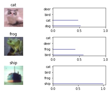
The model gives around 81% accuracy on the test set. I have an iPython notebook on my GitHub site that lets you load the saved model and run it on random samples on the test set. It outputs the image vs the softmax probabilities of the top n predictions.
