In recent years Recurrent Neural Networks have shown great results in NLP tasks – generating text, neural machine translation, question answering, and a lot more.
In this post we will explore text generation – teaching computers to write in a certain style. This is based off (and a recreation of) Andrej Karpathy’s famous article The Unreasonable Effectiveness of Recurrent Neural Networks.
Predicting the next character in a sentence is a language model problem. Traditionally these were done using n-gram models. For example a unigram model would be the distribution of individual characters. At each time step we would predict a character using that probability distribution. A bigram model would take the probability distribution of 2 characters (for example, given the first letter a, what is the probability of the second letter is n). Mathematically
![\[P(W_n|W_{n-1}) = \frac{P(W_{n-1},W_n)}{P(W_{n-1})}\]](http://rohitapte.com/wp-content/ql-cache/quicklatex.com-d5c2670adefae5d7d9cbe8b9fdd2cd21_l3.png "Rendered by QuickLaTeX.com")
Doing this at a word level has a disadvantage – how to handle out of vocabulary words. Character models don’t have this problem since they learn general distributions of the underlying text. However, the challenge with n-gram models (word and character) is that the memory required grows exponentially with each additional n. We therefore have a limit to how far back in a sequence we can look. In our example we use an alphabet size of 98 characters (small case and capital letters, and special characters like space, parenthesis etc). A bigram model would take have 9,604 possible letter pairs. With a trigram model it grows to 941,192 possible triplets. In our example we go back 30 characters. That would require us to store 5.46e59 possible combinations.
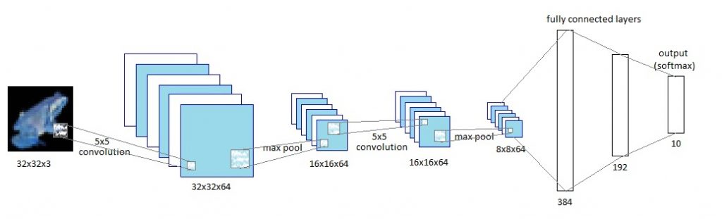
This is where we can leverage the use of RNNs. I’m assuming you have an understanding of LSTMs and I will only describe the network architecture here. There is an excellent article by Christopher Olah on understanding RNNs and LSTMs that goes into the details of the underlying math.
For this problem we take data in sequences of 30 characters and try to predict the next character for each letter. We are using stateful LSTMs – the data is fed in batches but each batch is a continuation of the previous one. We also save the state of the LSTM at the end of each batch and use this as the initial state for the next batch. The benefit of doing this is that the system can learn longer term dependencies like closing an open parenthesis or bracket, ending a sentence with a period, etc. The code is available on my GitHub, and you can tweak the model parameters to see how the results look.
The model is agnostic to the data. I ran it on 3 different datasets – Shakespeare, Aesop’s fables and a crawl of Paul Graham‘s website. The same code learns to write in each style after a few epochs. In each case, it learns formatting, which words are commonly used, to close open quotes and parenthesis, etc.
We generate sample data as follows – we sample a capital letter (“L” in our case) and then ask the RNN to predict the next letter. we take the n highest probabilities (2 in these examples, but its a parameter that can be adjusted) and generate the next letter. Using that letter we generate the next one, and so on. Here are samples of the data for each dataset.
Shakespeare – we can see that the model learns quickly. At the end of the first epoch its already learned to format the text, close parenthesis (past the 30 character input) and add titles and scenes. After 5 epochs it gets even better and at 60 epochs it generates very “Shakespeare like” text.
|
1 2 3 4 5 6 7 8 9 10 11 12 13 14 15 16 17 18 19 20 21 22 23 24 25 26 27 28 29 30 31 32 33 34 35 36 37 38 39 40 41 42 |
OLENTZA My large of my soul so more that I will Then then will not so. The king of my lord, and we would to the more and my lord, that the word of this hand And than this way to this, and to be my lord. [Exeunt] THE TONY VENCT IV SCENE I A part off. [Enter MARCUTES and Servant] TREISARD PERTINE, LARD LEND, LECE,) THE SARDINAND, and Antondance of Encarder to the pain and the part on the caption. [Exeunt MERCUS and SIR ANDRONICUS, LEONATUS] FARDINAL How now, so, my lord. [Enter MARCUS and MARIUS] Where is the stare? [Exeunt] THE TONY VELINE LENR ENT ACT II SCENE V I have her heart of the heaver to the part. [Enter LARIUS, and Sending] [Exeunt LACIUS, and Servants] Where is this would say you say, And where you have some thanks of this wild but Then we will not some many me thank you will That I would no more to my live to her the past of my hand. I would |
|
1 2 3 4 5 6 7 8 9 10 11 12 13 14 15 16 17 18 19 20 21 22 23 24 25 26 27 28 29 30 31 32 33 34 |
ANDORE With this the service of a servant to him, and the wind which hath been seen to take the countenance, the wind of thee and still to see his sine of him. [Exeunt LORD POLONIUS and LADY MACBETH] And so with you, my lord, I will not see The sun of thee that I have heard your sines. [Exit] [Enter a Senator of the world of Winchester] How now, my lord, the king of England say so says The season will be married to thy heart. Therefore, the king, that would have seen the sense Of the worst, that we will never see him. SILVIA I will not have her better than he hath seen. [Exeunt BARDOLPH, and Attendants] That hath my signior shall not speak to me, To say that I have have the crown of men And shall I have the strength of this my love. I hope they will, and see thee to thy heart that thou dost send The traitors of the state of thine, And shall the service to the constancy. [Exeunt] KING HENRY VI ACT III SCENE III A street of the part. |
|
1 2 3 4 5 6 7 8 9 10 11 12 13 14 15 16 17 18 19 20 21 22 23 24 25 26 27 28 29 30 31 32 33 34 35 36 37 |
[Enter another Messenger] Messenger Madam, I will not speak to them. CORDELIA I have a son of the person of the world. [Exit Servant] How now, Montague, What says the word of the foul discretion? The king has been a maiden short of him. [Exeunt] THE TWO GENTLEMEN OF VERONA ACT III SCENE II The forest. [Alarum. Enter KING LEAR, and others] KING HENRY VIII Then look upon the king and the street of the king, As the subject of my son is most deliver'd, And my the honest son of my honour, That I must see the king and tongue that shows That I have made them all as things as me. KING HENRY VIII What, will you see my heart and to my son? KING HENRY VI Why, then, I say an earl and the sense Who shall not stay the sun to heart to speak. I have not seen my heart, and shall be so. The king's son will not be a monster's son. [Exit] |
Paul Graham posts – we have about 80% less data compared to Shakespeare and his writing style is more “diverse” so the model doesn’t do as well after the first epoch. Words are often incomplete. After 5 epochs we see a significant improvement – most words and the language structure are correct. The writing style is starting to resemble Paul Graham. After 60 epochs we see a big improvement overall but still have issues with some nonsensical words.
|
1 2 3 4 5 6 7 8 9 10 11 12 13 14 15 16 17 18 |
They've deal in the for the sere the searse to work of the first the progetting the founders to be the founders. They're so exame the for to may be the finst a company. It's no have to grink to better who have to get the form to be a seal anyone with to griet to be the startup work to be. The fart a could be a startup wilh be they deal they work the strate they're the find on the straction that they would have to get the founders will be a stre finst invest the find that they was that the precest in an example who work to griet than you con'l your a startup work the serves to way to grow the first that they want to be a sear how and and the first people where the seee to be a lear how the first the perple the sere the first perple will be an exter is to be to be the serves the first that they'll the founders when you can't was any deal the four examply, and you can de a startup with to growth that while that's the prectice the seal a find the sere they want the for a seart prese |
|
1 2 3 4 5 6 7 8 9 10 11 12 13 14 15 16 17 18 19 20 21 22 |
It's not sure they were something that they're supposed to be a lot of things. The risk of the problems is a startup. It's that they wanted to be too much to them and seem to be the product valuation of the street that would be a lot of people to seem that they could be able to do that. It's the same problems to start a startup is an idea of the product valuetion of a startup in the companies to start a series. And that seens the press of a startup to be able to do it to start a startup in the same. It would become things that wants to be the big commany. The problem with a strett is a startup is that they're also being a straight of a smart startup ideas. The problem is that they're all to do it. It's the same thing to be some kind of person that was a lot of people who are to seem to be a lot of people to start any startup. They're so much that's what they're a large problem is to be the structural offer and the problem is the startup ideas. It's the sacrisical company they |
|
1 2 3 4 5 6 7 8 9 10 11 12 13 14 15 16 17 18 19 20 21 22 23 24 25 26 27 28 |
The programing language is the problem with the product than a lot of people to start a startup in the same. If you want to get the people you'll have a large pattern of an advantage, you can start to get a startup. It's not just the same thing that could be able to start a startup is the same patents. It's not as a sign that it's not just the biggest stagtup ideas. They won't get them a lot of them and the best startups to sell to a starting to build a series A round. The reason I think it's the same. If the fundamental person to do that, the best people are also trying to do it will tend to be the same time. This was the part of the first time they can do to start the startups than they wanted. They're also the only way to get a lot of people who want to do it. They'll be able to seem to be a great deal to start a startup that startups will succeed as a significant company. It won't seem a lot of people to be so much that it would be. The people are so close that they were already true that they were a list of the same problems. They can't see the rest of their prevertions. To this control of startups are the same time and all they could get to the standard of a startup than they were startups. They won't believe it that's the serioss of their own startups. The people are a lot of the problem to start a startup to be the second is that it seems to be a good idea. |
Aesop’s fables – the dataset is quite small so the model takes a lot longer to train. But it also gives us an insight into how the RNN is learning. After 1 epoch it only learns the more common letters in the language. It took 15 epochs for it to start to put words together. After 60 epochs it does better, but still has non English words. But it does learn the writing style (animal names in capital, different formatting from the above examples, etc).
|
1 2 3 4 5 6 7 8 9 10 11 12 13 14 15 16 17 18 19 20 |
ee e oo ttt tt ttt e e e eeee e ee e ee e ee e eee eeee e e e eee eeee ee ee e ee ee ee e ee e e ee e e ee e ee e ee e eeee eeee ee e e eeee eeee ee e ee e ee ee ee e e ee e e ee e e e e eeee ee e e e e e ee ee ee eeee e ee eee eee ee eee e e eeee e e eeeee ee ee e e e e ee ee ee ee e e e e e ee e ee ee ee e eeeeee e e ee e e e e e ee e e eeeee e ee ee ee e e e e ee ee e e e e eee eeee ee ee e ee e ee e e e e e ee eeee e ee eeeee e e e ee ee eee eee e eeee eee e e ee e e e e e e e e ee eee e eeee ee ee ee e ee e e e e e e ee e e eeeee ee e e e eee e e ee ee eeee ee ee e eee e ee e e e ee e eeeee e e eeee ee ee eeeee e e eee e ee ee e e ee e ee ee eee e e e e ee ee eee ee e eeeeee e e e |
|
1 2 3 4 5 6 7 8 9 10 11 12 13 14 15 16 17 18 19 20 21 22 |
"The Horse and the Fox and and to the bound and and the sard to the boute r and and andered than to to him to he pare. "I a pang a bound the Fox, and shat the Lound the boun the sored and the sout the Lound and to ther the wint the boune and the sore to his his. An he coned than the sand the sound and and apled the Hore ander the soon the sord his his to care an tor him t he bound the bout." A Fan a cane a biged, a pard an a piged to him him his the pound an and and tor and to the sore an that her wan to the bore and ander the sore. The Louted and the porned than her was to the sare. The Loun to he sain the bound the porned to to here to to his here and anded and and apling to the boune ander and the south the sore. Then his her ase and the Laon to the bon that he cand the porned the berter. The Ling the bon the pare an a pored the Hores the bene to his her as andered the Horser. An that then the Loond to to he parder and then was his to his his he care the bou |
|
1 2 3 4 5 6 7 8 9 10 11 12 13 14 15 16 17 18 19 |
Then he took his back in their tails, and gave his to a prace, and suppesed, and threw his bitter than hapeled that he would not injore the mirk where the wheels said: "I would gave a ply on the road, and that I have nothor you can ot ereath this tise to put out that he right horring towards the right. When he came herd on the brance of the Bod had to give him a pignt of the Fox wert string themselves began to carry him and he had his closs, and brew him to his mouth of his coutin, but soon stopped the Hart was successing them the Fox intited the Stork to the Lion, we tould having his to himself the Lag once decaired it into the Pitcher. At last, and stop and did the time of his boy of the Frogs, lifting his horns and suck unto dis and played up to him peck of his break. "I have a sholl borst with the reach of the roges of too ore that he was doint down to his mach, a smanl day which the hand of her hounds and soon had to give them with his not like to her some in the country. |
The source code is available on my GitHub for anyone who wants to play with it. Please make sure you have a GPU with CUDA and CUDNN installed, otherwise it will take forever to train. The model parameters can be changed using command line arguments.
I also added a file in the git called n-gram_model.py that lets you try the same exercise with n-grams to compare how well the deep learning method does vs different n-gram sizes (both speed and accuracy).