CIFAR-10 is an established computer vision dataset used for image recognition. Its a subset of 80 million tiny images collected by Alex Krizhevsky, Vinod Nair, and Geoffrey Hinton. This is the link to the website.
The CIFAR-10 dataset consists of 60,000 32×32 color images of 10 classes, with 6,000 images per class. There are 50,000 training images and 10,000 test images.
As a first post, I wanted to write a deep learning algorithm to identify images in the CIFAR-10 database. This topic has been very widely covered – in fact Google’s Tensorflow tutorials cover this very well. However, they do a few things that made it difficult for me to follow their code
- They split the code across multiple files making it difficult to follow.
- They use a binary version of the file and a file stream to feed Tensorflow.
I downloaded the python version of the data and loaded all the variables into memory. There is some image manipulation done in the tensorflow tutorial that I recreated in the numpy arrays directly and we will discuss it below.
Prerequisites for this tutorial:
Other than Python (obviously!)
- numpy
- pickle
- sklearn
- tensorflow
For TensorFlow I strongly recommend the GPU version if you have the set-up for it. The code takes 6 hours on my dual GTX Titan X machine and running it on a CPU will probably take days or weeks!
Assuming you have everything working, lets get started!
Start with our import statements
|
|
import numpy as np import pickle from sklearn import preprocessing import random import math import os from six.moves import urllib import tarfile import tensorflow as tf |
Declare some global variables we will use. In our code we are using GradientDescentOptimizer with learning rate decay. I have tested the same code with the AdamOptimizer. Adam runs faster but gives slightly worse results. If you do decide to use the AdamOptimizer, drop the learning rate to 0.0001. This is the link to the paper on Adam optimization.
|
|
NUM_FILE_BATCHES=5 LEARNING_RATE = 0.1 LEARNING_RATE_DECAY=0.1 NUM_GENS_TO_WAIT=250.0 TRAINING_ITERATIONS = 30000 DROPOUT = 0.5 BATCH_SIZE = 500 IMAGE_TO_DISPLAY = 10 |
Create data directory and download data if it doesn’t exist – this code will not run if we have already downloaded the data.
|
|
data_dir='data' if not os.path.exists(data_dir): os.makedirs(data_dir) cifar10_url='https://www.cs.toronto.edu/~kriz/cifar-10-python.tar.gz' data_file=os.path.join(data_dir, 'cifar-10-binary.tar.gz') if os.path.isfile(data_file): pass else: def progress(block_num, block_size, total_size): progress_info = [cifar10_url, float(block_num * block_size) / float(total_size) * 100.0] print('\r Downloading {} - {:.2f}%'.format(*progress_info), end="") filepath, _ = urllib.request.urlretrieve(cifar10_url, data_file, progress) tarfile.open(filepath, 'r:gz').extractall(data_dir) |
Load data into numpy arrays. The code below loads the labels from the batches.meta file, and the training and test data. The training data is split across 5 files. We also one hot encode the labels.
1 2 3 4 5 6 7 8 9 10 11 12 13 14 15 16 17 18 19 20 21 22 23 24 25 26 27 |
with open('data/cifar-10-batches-py/batches.meta',mode='rb') as file: batch=pickle.load(file,encoding='latin1') label_names=batch['label_names'] def load_cifar10data(filename): with open(filename,mode='rb') as file: batch=pickle.load(file,encoding='latin1') features=batch['data'].reshape((len(batch['data']),3,32,32)).transpose(0,2,3,1) labels=batch['labels'] return features,labels x_train=np.zeros(shape=(0,32,32,3)) train_labels=[] for i in range(1,NUM_FILE_BATCHES+1): ft,lb=load_cifar10data('data/cifar-10-batches-py/data_batch_'+str(i)) x_train=np.vstack((x_train,ft)) train_labels.extend(lb) unique_labels=list(set(train_labels)) lb=preprocessing.LabelBinarizer() lb.fit(unique_labels) y_train=lb.transform(train_labels) x_test_data,test_labels=load_cifar10data('data/cifar-10-batches-py/test_batch') y_test=lb.transform(test_labels) |
Having more training data can improve our algorithms. Since we are confined to 50,000 training images (5,000 for each category) we can “manufacture” more images using small image manipulations. We do 3 transformations – flip the image horizontally, randomly adjust the brightness and randomly adjust the contrast. We also normalize the data. Note that there are different ways to do this, but standardization works best for image. However rescaling can be an option as well.
1 2 3 4 5 6 7 8 9 10 11 12 13 14 15 16 17 18 19 20 21 |
def updateImage(x_train_data,distort=True): x_temp=x_train_data.copy() x_output=np.zeros(shape=(0,32,32,3)) for i in range(0,x_temp.shape[0]): temp=x_temp[i] if distort: if random.random()>0.5: temp=np.fliplr(temp) brightness=random.randint(-63,63) temp=temp+brightness contrast=random.uniform(0.2,1.8) temp=temp*contrast mean=np.mean(temp) stddev=np.std(temp) temp=(temp-mean)/stddev temp=np.expand_dims(temp,axis=0) x_output=np.append(x_output,temp,axis=0) return x_output #update test data since we don't have to apply distortions #for training data for each batch we will randomly distory before normalizing x_test=updateImage(x_test_data,False) |
Now comes the fun part. This is what our network looks like.

Lets define the various layers of the network. The last line of code (logits=tf.identity(final_output,name=’logits’)) is done in case you want to view the model in TensorBoard.
1 2 3 4 5 6 7 8 9 10 11 12 13 14 15 16 17 18 19 20 21 22 23 24 25 26 27 28 29 30 31 32 33 34 35 36 37 38 39 40 41 42 43 44 45 46 47 48 49 50 51 52 53 54 55 56 |
def truncated_normal_var(name, shape, dtype): return(tf.get_variable(name=name, shape=shape, dtype=dtype, initializer=tf.truncated_normal_initializer(stddev=0.05))) def zero_var(name, shape, dtype): return(tf.get_variable(name=name, shape=shape, dtype=dtype, initializer=tf.constant_initializer(0.0))) x=tf.placeholder(tf.float32,shape=[None,x_train.shape[1],x_train.shape[2],x_train.shape[3]],name='x') labels=tf.placeholder(tf.float32,shape=[None,y_train.shape[1]],name='labels') keep_prob=tf.placeholder(tf.float32,name='keep_prob') with tf.variable_scope('conv1') as scope: conv1_kernel=truncated_normal_var(name='conv1_kernel',shape=[5,5,3,64],dtype=tf.float32) strides=[1,1,1,1] conv1=tf.nn.conv2d(x,conv1_kernel,strides,padding='SAME') conv1_bias=zero_var(name='conv1_bias',shape=[64],dtype=tf.float32) conv1_add_bias=tf.nn.bias_add(conv1,conv1_bias) relu_conv1=tf.nn.relu(conv1_add_bias) pool_size=[1,3,3,1] strides=[1,2,2,1] pool1=tf.nn.max_pool(relu_conv1,ksize=pool_size,strides=strides,padding='SAME',name='pool_layer1') norm1=tf.nn.lrn(pool1,depth_radius=4,bias=1.0,alpha=0.001/9.0,beta=0.75,name='norm1') with tf.variable_scope('conv2') as scope: conv2_kernel=truncated_normal_var(name='conv2_kernel',shape=[5,5,64,64],dtype=tf.float32) strides=[1,1,1,1] conv2=tf.nn.conv2d(norm1,conv2_kernel,strides,padding='SAME') conv2_bias=zero_var(name='conv2_bias',shape=[64],dtype=tf.float32) conv2_add_bias=tf.nn.bias_add(conv2,conv2_bias) relu_conv2=tf.nn.relu(conv2_add_bias) pool_size=[1,3,3,1] strides=[1,2,2,1] pool2=tf.nn.max_pool(relu_conv2,ksize=pool_size,strides=strides,padding='SAME',name='pool_layer2') norm2=tf.nn.lrn(pool2,depth_radius=4,bias=1.0,alpha=0.001/9.0,beta=0.75,name='norm2') reshaped_output=tf.reshape(norm2, [-1, 8*8*64]) reshaped_dim=reshaped_output.get_shape()[1].value with tf.variable_scope('full1') as scope: full_weight1=truncated_normal_var(name='full_mult1',shape=[reshaped_dim,1024],dtype=tf.float32) full_bias1=zero_var(name='full_bias1',shape=[1024],dtype=tf.float32) full_layer1=tf.nn.relu(tf.add(tf.matmul(reshaped_output,full_weight1),full_bias1)) full_layer1=tf.nn.dropout(full_layer1,keep_prob) with tf.variable_scope('full2') as scope: full_weight2=truncated_normal_var(name='full_mult2',shape=[1024, 256],dtype=tf.float32) full_bias2=zero_var(name='full_bias2',shape=[256],dtype=tf.float32) full_layer2=tf.nn.relu(tf.add(tf.matmul(full_layer1,full_weight2),full_bias2)) full_layer2=tf.nn.dropout(full_layer2,keep_prob) with tf.variable_scope('full3') as scope: full_weight3=truncated_normal_var(name='full_mult3',shape=[256,IMAGE_TO_DISPLAY],dtype=tf.float32) full_bias3=zero_var(name='full_bias3',shape=[IMAGE_TO_DISPLAY],dtype=tf.float32) final_output=tf.add(tf.matmul(full_layer2,full_weight3),full_bias3,name='final_output') logits=tf.identity(final_output,name='logits') |
Now we define our cross entropy and optimization function. If you want to use the AdamOptomizer, uncomment that line, comment the generation_run, model_learning_rate and train_step lines and adjust the learning rate to something lower like 0.0001. Otherwise the model will not converge.
|
|
cross_entropy=tf.reduce_mean(tf.nn.softmax_cross_entropy_with_logits(logits=logits,labels=labels),name='cross_entropy') #train_step=tf.train.AdamOptimizer(LEARNING_RATE).minimize(cross_entropy) generation_run = tf.Variable(0, trainable=False,name='generation_run') model_learning_rate=tf.train.exponential_decay(LEARNING_RATE,generation_run,NUM_GENS_TO_WAIT,LEARNING_RATE_DECAY,staircase=True,name='model_learning_rate') train_step=tf.train.GradientDescentOptimizer(LEARNING_RATE).minimize(cross_entropy) correct_prediction=tf.equal(tf.argmax(final_output,1),tf.argmax(labels,1),name='correct_prediction') accuracy=tf.reduce_mean(tf.cast(correct_prediction,tf.float32),name='accuracy') |
Now we define some functions to run through our batch. For large networks memory tends to be a big constraint. We run through our training data in batches. One epoch is one run through our complete training set (in multiple batches). After each epoch we randomly shuffle our data. This helps improve how our algorithm learns. We run through each batch of data and train our algorithm. We also check for accuracy every 1st, 2nd,…,10th, 20th,…, 100th,… step. Lastly we calculate the final accuracy of the model and save it so we can use the calculated weights on test data without having to re-run it.
1 2 3 4 5 6 7 8 9 10 11 12 13 14 15 16 17 18 19 20 21 22 23 24 25 26 27 28 29 30 31 32 33 34 35 36 37 38 39 40 41 42 43 44 45 |
epochs_completed=0 index_in_epoch = 0 num_examples=x_train.shape[0] init=tf.global_variables_initializer() with tf.Session() as sess: sess.run(init) def next_batch(batch_size): global x_train global y_train global index_in_epoch global epochs_completed start = index_in_epoch index_in_epoch += batch_size if index_in_epoch > num_examples: # finished epoch epochs_completed += 1 # shuffle the data perm = np.arange(num_examples) np.random.shuffle(perm) x_train=x_train[perm] y_train=y_train[perm] # start next epoch start = 0 index_in_epoch = batch_size assert batch_size <= num_examples end = index_in_epoch #return x_train[start:end], y_train[start:end] x_output=updateImage(x_train[start:end],True) return x_output,y_train[start:end] # visualisation variables train_accuracies = [] validation_accuracies = [] x_range = [] display_step=1 for i in range(TRAINING_ITERATIONS): #get new batch batch_xs, batch_ys = next_batch(BATCH_SIZE) # check progress on every 1st,2nd,...,10th,20th,...,100th... step if i%display_step == 0 or (i+1) == TRAINING_ITERATIONS: train_accuracy = accuracy.eval(feed_dict={x:batch_xs,labels: batch_ys,keep_prob: 1.0}) validation_accuracy=0.0 for j in range(0,x_test.shape[0]//BATCH_SIZE): validation_accuracy+=accuracy.eval(feed_dict={ x: x_test[j*BATCH_SIZE : (j+1)*BATCH_SIZE],labels: y_test[j*BATCH_SIZE : (j+1)*BATCH_SIZE],keep_prob: 1.0}) validation_accuracy/=(j+1.0) print('training_accuracy / validation_accuracy => %.2f / %.2f for step %d'%(train_accuracy, validation_accuracy, i)) validation_accuracies.append(validation_accuracy) train_accuracies.append(train_accuracy) x_range.append(i) # increase display_step if i%(display_step*10) == 0 and i: display_step *= 10 # train on batch sess.run(train_step, feed_dict={x: batch_xs, labels: batch_ys, keep_prob: DROPOUT}) validation_accuracy=0.0 for j in range(0,x_test.shape[0]//BATCH_SIZE): validation_accuracy+=accuracy.eval(feed_dict={ x: x_test[j*BATCH_SIZE : (j+1)*BATCH_SIZE],labels: y_test[j*BATCH_SIZE : (j+1)*BATCH_SIZE],keep_prob: 1.0}) validation_accuracy/=(j+1.0) print('validation_accuracy => %.4f'%validation_accuracy) saver=tf.train.Saver() save_path=saver.save(sess,'./CIFAR10_model') sess.close() |
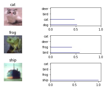
The model gives around 81% accuracy on the test set. I have an iPython notebook on my GitHub site that lets you load the saved model and run it on random samples on the test set. It outputs the image vs the softmax probabilities of the top n predictions.

![]()
 Some more intuitive explanations of convolutions (and more applicable to machine learning):
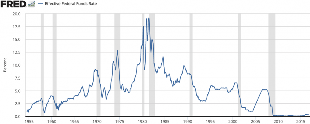 One way to smooth data is to convolve it against a smaller list. For example, to calculate the weekly moving average we convolve it against [1,1,1,1,1]. For a monthly moving average we would convolve it with a list of 25 ones (assuming 25 business days in a month).
 This can be represented as a convolution… For example to get a 4 we have

