I gave a talk at the Hong Kong Machine Learning Meetup on 17th April 2019. These are the slides from that talk.
Stylometric analysis of Emails
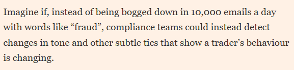
There was an FT article recently (25th March 2019) on Banks using AI to catch rogue traders before the act. The second paragraph stood out for me –
How would one go about tackling something like this? We would use something called Stylometry. Stylometry is often used to attribute authorship to anonymous or disputed documents. In this post we will try and apply Stylometry to emails to see if we can identify the writer.
Due to privacy issues, its not easy to get a dataset of email conversations. The one that I managed to find was the Enron Email Dataset which contains over 500,000 emails generated by employees of Enron. It was obtained by the Federal Energy Regulatory Commission during its investigation of Enron’s collapse.
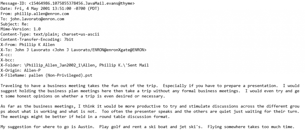
The Enron dataset contains emails in MIME format. This is what a sample email looks like
I took the emails and stripped them of any forwarded or replied to text, and disclaimers to preserve only what the person actually wrote. This is important since we are analyzing writing style. I also added the option to filter by messages of a minimum length (more on that later). Lastly I restricted the analysis to the 10 most active people in the dataset.
| kay.mann@enron.com | vince.kaminski@enron.com |
| jeff.dasovich@enron.com | chris.germany@enron.com |
| sara.shackleton@enron.com | tana.jones@enron.com |
| eric.bass@enron.com | matthew.lenhart@enron.com |
| kate.symes@enron.com | sally.beck@enron.com |
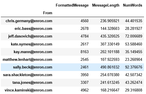
We get just over 40,000 emails with a decent distribution across all the people. An analysis of the average length and number of words for each person already shows us that each person is quite different in how they write emails.
For our analysis we will split the data into training and test sets, apply Stylometric analysis to the training data and use it to predict the test data.
For Stylometric analysis I used John Burrow’s delta method. Published in 2002, it is a widely used and accepted method to analyze authorship. Here are the steps for calculating the delta
- Take the entire corpus (our training set) and find the n most frequent words.
- Calculate the probability of each of these words occurring in the entire corpus (freq distribution of the word/total words in the corpus).
- Calculate the mean and standard deviation of the occurrence of the word for each author.
- Calculate the z-scores for every word for every author.
- For the text in the test set, calculate the probabilities of the frequent words and their z-scores.
- The delta = Sum of absolute value of difference in z scores divided by n.
- The smallest delta is the one we predict to be the author.
What do the results look like? Overall, pretty good considering we are trying to classify emails as belonging one of 10 possible authors with very little data (usually one identifies the author for a book, and has a large corpus to generate word frequencies). For example, it automatically picks up the fact that someone tends to use quotes a lot
Author: jeff.dasovich@enron.com
Email: I’d like to do everything but the decking for the deck. We can hold off on that.
In addition, I may have some “salvaged” redwood decking I may want to add to the mix once I get ready to install the decking.
Best, Jeff
Scores: {‘kay.mann@enron.com’: 7.43433684056309, ‘vince.kaminski@enron.com’: 7.337718602815618, ‘jeff.dasovich@enron.com’: 7.056721256733514, ‘chris.germany@enron.com’: 7.522215636238818, ‘sara.shackleton@enron.com’: 7.5393982224001945, ‘tana.jones@enron.com’: 7.434437992786343, ‘eric.bass@enron.com’: 7.54634308986968, ‘matthew.lenhart@enron.com’: 7.517654790021831, ‘kate.symes@enron.com’: 7.624201059391151, ‘sally.beck@enron.com’: 7.548497152341907}
Author: kay.mann@enron.com
Email: I have a couple of questions so I can wrap up the LOI:
We refer to licensed Fuel Cell Energy equipment. Do we intend to reference a particular manufacturer, or should this be more generic?
Do we want to attach a draft of the Development Agreement, and condition the final deal on agreeing to terms substantially the same as what’s in the draft? I have a concern that the Enron optionality bug could bite us on the backside with that one.
Do we expect to have ONE EPC contract, or several?
I’m looking for the confidentiality agreement, which may be in Bart’s files (haven’t checked closely yet). If anyone has it handy, it could speed things up for me.
Thanks, Kay
{‘kay.mann@enron.com’: 6.154191709401956, ‘vince.kaminski@enron.com’: 6.397433577625913, ‘jeff.dasovich@enron.com’: 6.396576407146207, ‘chris.germany@enron.com’: 6.642765292897169, ‘sara.shackleton@enron.com’: 6.56876557432365, ‘tana.jones@enron.com’: 6.249601335542451, ‘eric.bass@enron.com’: 6.595756852792294, ‘matthew.lenhart@enron.com’: 6.7300358896137595, ‘kate.symes@enron.com’: 6.4104713094426815, ‘sally.beck@enron.com’: 6.318539264208084}
The predictions tend to do better on longer emails. On smaller emails as well as emails that don’t betray a writing style it doesn’t do a very good job. For example
Author: chris.germany@enron.com
Email: Please set up the following Service Type, Rate Sched combinations.
Pipe Code EGHP
Firmness Firm
Service Type Storage
Rate Sched FSS
Term Term
thanks
Scores: {‘kay.mann@enron.com’: 8.032067481552536, ‘vince.kaminski@enron.com’: 7.686060503779472, ‘jeff.dasovich@enron.com’: 7.76376151369006, ‘chris.germany@enron.com’: 8.088435461708675, ‘sara.shackleton@enron.com’: 7.837802283010304, ‘tana.jones@enron.com’: 8.356182289848462, ‘eric.bass@enron.com’: 8.285958154167018, ‘matthew.lenhart@enron.com’: 8.502751475726505, ‘kate.symes@enron.com’: 8.061320580331817, ‘sally.beck@enron.com’: 8.535085342764473}
How does filtering for longer emails affect our accuracy? How do we measure accuracy across the entire test set? I stole a page from the Neural Network playbook.
- Take the negative of our delta score (negative because lower is better).
- Apply SoftMax to convert it to probabilities.
- Calculate the cross entropy log loss.
Overall we do see an improvement filtering for larger emails but not by a much. This is partly because Burrow’s delta is quite stable and works on smaller datasets, as well as due to nuances in the Enron data.
| Minimum words | Cross Entropy Log Loss |
| 0 | 18.40066081813624 |
| 10 | 18.356774963612363 |
| 20 | 18.309804439201955 |
| 30 | 18.30380323248317 |
| 40 | 18.282598926893684 |
| 50 | 18.291281635444992 |
| 60 | 18.292350501846915 |
| 70 | 18.299773312100324 |
| 80 | 18.29375907006795 |
| 90 | 18.26679623872471 |
How can we adapt this to what the FT described? Given enough training data (emails from a trader) we can establish a baseline style (use of words, sentence length, etc.) and check for variations from that baseline. More than 2 standard deviations from that baseline could warrant a more closer look. If we have historical data of when rogue behavior occurred, we could use that to train our features to determine which one are better predictors for this change in behavior.
Source code for this project can be found on my GitHub. You will need to download the Enron email data file (link on my git) for the code to work.
An analysis of Tesla Tweets
Love it or hate it Tesla as a company draws some very polarized opinions. Twitter is full of arguments both for and against the company. In this post we will see how to tackle this from an NLP perspective.
Disclaimer: This article is intended to purely show how to tackle this from an NLP perspective. I am currently short Tesla through stocks and options and any data and results presented here should not be interpreted as research or trading advice.
Fetching Twitter data
There are many libraries out there to fetch twitter data. The one I used was tweepy. I downloaded 25,000 of the most recent tweets and filtered for tweets in English. We were left with 18,171 tweets over a period of 9 days. Tweepy has a few configurable options. Unless you have a paid subscription you need to account for Rate Limiting. I also chose to filter out retweets and selected extended mode to get the full text of each tweet.
|
1 2 3 4 |
auth = tweepy.OAuthHandler(consumer_key, consumer_secret) auth.set_access_token(access_token, access_token_secret) api = tweepy.API(auth, wait_on_rate_limit=True) search_hashtag = tweepy.Cursor(api.search, q="TSLA -filter:retweets",tweet_mode='extended').items(25000) |
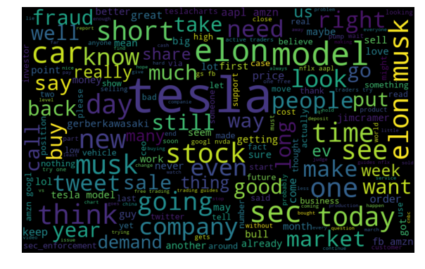
No NLP post is complete without a word cloud! We generate one on the twitter text removing stop words and punctuations. Its an interesting set of words – both positive and negative.
Sentiment Analysis
I found Vader (Valence Aware Dictionary and sEntiment Reasoner) to be a very good tool for Twitter sentiment analysis. It uses a lexicon and rule-based approach especially attuned to sentiments expressed in social media. Vader returns a score of 1 split across positive, neutral and and a compound score between -1 (extremely negative) and +1 (extremely positive). We use the compound score for our analysis. Here are the results for some sample tweets that it got correct.
|
1 2 3 4 5 6 7 8 9 10 |
If there was no fraud, there was no demand issue, no cash crunch, this is what would kill Tesla. Crafting artisan cars in the most expensive part of the world while competition is virtually fully automated already simply can't fly. Compound score: -0.9393 @GerberKawasaki Generational opportunity GERBER to add to TSLA longs. This might be the last chance to get in before she blows! Compound score: 0.6239 |
Vader gets plenty of classifications wrong. I guess the language for a stock is quite nuanced.
|
1 2 3 4 5 6 7 8 9 10 |
Today in "a company that is absolutely not experiencing a cash crunch". $TSLA Compound score: 0.0 Tesla (TSLA) Stock Ends the Week in Red. Are the Reasons Model Y or Musk Himself? #cryptocurrency #btcnews #altcoins #enigma #tothemoon #altcoins #pos Compound score: 0.0 Tesla (TSLA:NAS) and China Unicom (CHU:NYS) Upgraded Compound score: 0.0 |
One option is to train our own sentiment classifier if we can find a way to label data. But what about clustering tweets and analyzing sentiment by cluster? We may get a better understanding of which ones are classified correctly that way.
To cluster tweets we need to vectorize them so we can compute a distance metric. TFIDF works very well for this task. TFIDF consists of 2 components
Term Frequency – how often a word occurs in a document
Inverse Document Frequency – how much information the word provides (whether its common or rare across all documents).
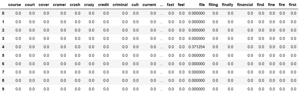
Before applying TFIDF we need to tokenize our words. I used NLTK’s TweetTokenizer which preserves mentions and $ tags, and lemmatized the words to collapse similar meaning words (we could also try stemming). I also removed all http links in tweets since we cant analyze them algorithmically. Finally I added punctuations to the stop words that TFIDF will ignore. I ran TFIDF using 1000 features. This is a parameter that we can experiment with and tune. This is what a sample subset of resultant matrix looks like.
We finally have a matrix we can use to run KMeans. Determining the number of clusters is a frequently encountered problem in clustering, different from the process of actually clustering the data. I used the Elbow Method to fine tune this parameter – essentially we try a range of clusters and plot the SSE (Sum of Squared Errors). SSE tends to 0 as we increase the cluster count. Plotting the SSE against number of errors tends to have the shape of an arm with the “elbow” suggesting at what value we start to see diminishing reduction in SSE. We pick the number of clusters to be at the elbow point.
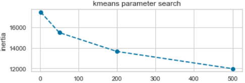
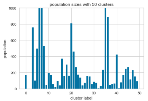
I decided to use 50 clusters since that’s where the elbow is. Its worth looking at a distribution of tweets for each cluster center and the most important features for clusters with a high population.
|
1 2 3 |
Cluster 6: ’ @elonmusk tesla elon ‘ musk stock #tesla sec time let going think today @tesla Cluster 7: @elonmusk #tesla @tesla stock time today would going cars short car company see day get Cluster 36: musk elon sec tesla ceo judge tweets contempt settlement via cramer going tesla's get |
Finally, to visualize the clusters we first use TSNE to reduce the TFIDF feature matrix to 2 dimensions, and then plot them using Bokeh. Bokeh lets us look at data when we hover over points to see how the clustering is working with text.
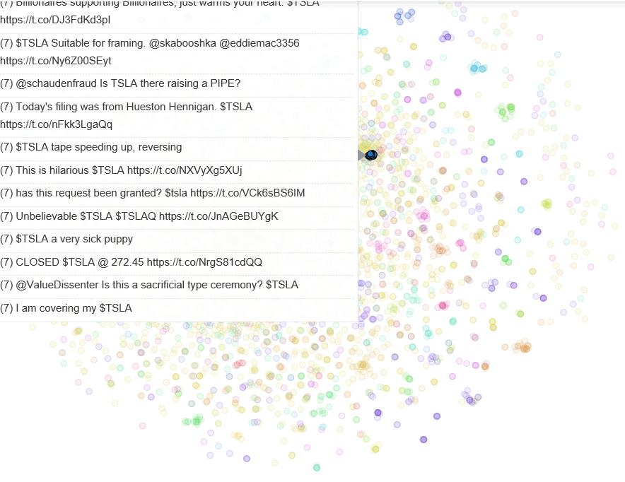
Analyzing the tweets and clusters I realized there is a lot of SPAM in twitter. For cleaner analysis its worth researching how to remove these tweets.
As usual, code is available on my Github.
Introduction to NLP
I recently gave a talk at a Hackathon on an introduction to Natural Language Processing. These are the slides from that talk.
K-Means for image compression
I recently finished Andrew Ng’s CS229 course remotely. The course was extremely challenging and covered a wide range of Machine Learning concepts. Even if you have worked with, and used Machine Learning algorithms, he introduced concepts in novel and interesting ways I didn’t expect. One of the things that struct a chord with me was how we worked on K-Means clustering.
The algorithm is quite simple. Courtesy of CS229…
Given a training set, if we want to group it into n clusters
![\[\{ x^{(1)},\cdots,x^{(m)} \} \]](http://rohitapte.com/wp-content/ql-cache/quicklatex.com-9617c9b9f5d4db0a48f733823813aace_l3.png "Rendered by QuickLaTeX.com")
1. Initialize cluster centroids randomly
![\[ \mu_1,\mu_2,\cdots,\mu_k \in \mathbb{R}^n \]](http://rohitapte.com/wp-content/ql-cache/quicklatex.com-707cb1244cd56d1a31b553dccb5b6d46_l3.png "Rendered by QuickLaTeX.com")
2. Repeat until convergence
For every i set
![\[ c^{(i)} := \arg \min_{j} ||x_{(i)}-\mu_j||^2 \]](http://rohitapte.com/wp-content/ql-cache/quicklatex.com-8521cbcd13bc3a4a1c2ac5d9022f9281_l3.png "Rendered by QuickLaTeX.com")
For each j set
![\[ \mu_j := \frac{\sum_{i=1}^{m}1 \{c^{(i)}=j \} x^{(i)}}{\sum_{i=1}^{m}1 \{ c^{(i)}=j \}} \]](http://rohitapte.com/wp-content/ql-cache/quicklatex.com-8d545cc2d1b8f3b92c1d831019ad1953_l3.png "Rendered by QuickLaTeX.com")
Here an example of running K-means on the Iris dataset.
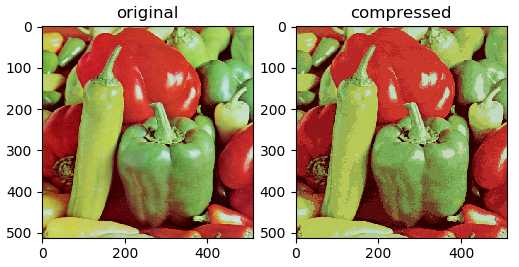
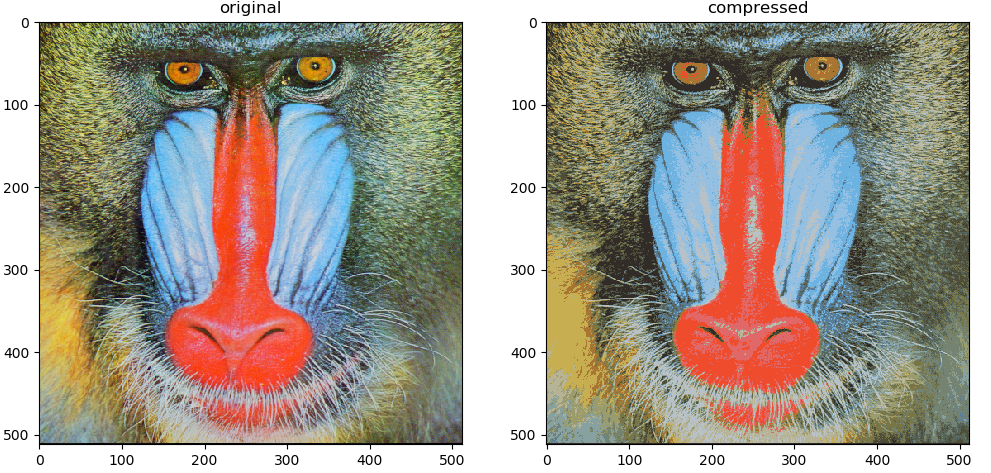
But an alternate use for K-Means is image compression. Given an image with the standard RGB colors we have 256x256x256=16.77M colors. We can use K-Means to compress these into less colors. The idea is similar to the above, with a few differences.
- We take an image of dimension (m,n,3) (3=R,G,B) and resize it to (mxn,3)
- For k clusters, we randomly sample k points from this data
- We assign colors closest to the k points we’ve selected to that cluster
- The new cluster points are the mean R,G,B points for each cluster
- We repeat this process until convergence (points don’t change, or we reach a threshold)
This is what the code looks like
|
1 2 3 4 5 6 7 8 9 10 11 12 13 14 15 16 17 18 19 20 21 22 23 24 25 26 27 28 29 30 31 32 33 34 35 |
def k_means_code(X,num_clusters): min_iters=30 X_reshaped=X.reshape(-1,3) #this variable will get resized past_min_indices =np.zeros(X_reshaped.shape[0]) # first set centroids to random points initial_indices=np.random.choice(X_reshaped.shape[0],num_clusters, replace=False) centroids=X_reshaped[initial_indices] #convert to float to prevent rounding on the averages centroids=centroids.astype(float) i=1 bContinueRunning=True while bContinueRunning: distances=np.array((0,0)) for centroid_index,centroid in enumerate(centroids): distance=np.sqrt(np.sum((X_reshaped - centroid) ** 2, axis=1)) if centroid_index==0: distances=distance.copy() else: distances=np.vstack((distances,distance)) min_indices=distances.argmin(axis=0) if np.sum(min_indices-past_min_indices)==0: bContinueRunning=False else: past_min_indices=min_indices.copy() for centroid_index in range(num_clusters): x_indices_in_centroid = np.where(min_indices == centroid_index)[0] X_in_centroid = X_reshaped[x_indices_in_centroid] centroids[centroid_index] = X_in_centroid.mean(axis=0) i+=1 if i>min_iters: print("Exceeded 30") bContinueRunning=False return centroids |
We can run this on a few images, reducing them from 16.77m colors to 16 colors to see how good the compression is
Character level language models using Recurrent Neural Networks
In recent years Recurrent Neural Networks have shown great results in NLP tasks – generating text, neural machine translation, question answering, and a lot more.
In this post we will explore text generation – teaching computers to write in a certain style. This is based off (and a recreation of) Andrej Karpathy’s famous article The Unreasonable Effectiveness of Recurrent Neural Networks.
Predicting the next character in a sentence is a language model problem. Traditionally these were done using n-gram models. For example a unigram model would be the distribution of individual characters. At each time step we would predict a character using that probability distribution. A bigram model would take the probability distribution of 2 characters (for example, given the first letter a, what is the probability of the second letter is n). Mathematically
![\[P(W_n|W_{n-1}) = \frac{P(W_{n-1},W_n)}{P(W_{n-1})}\]](http://rohitapte.com/wp-content/ql-cache/quicklatex.com-d5c2670adefae5d7d9cbe8b9fdd2cd21_l3.png "Rendered by QuickLaTeX.com")
Doing this at a word level has a disadvantage – how to handle out of vocabulary words. Character models don’t have this problem since they learn general distributions of the underlying text. However, the challenge with n-gram models (word and character) is that the memory required grows exponentially with each additional n. We therefore have a limit to how far back in a sequence we can look. In our example we use an alphabet size of 98 characters (small case and capital letters, and special characters like space, parenthesis etc). A bigram model would take have 9,604 possible letter pairs. With a trigram model it grows to 941,192 possible triplets. In our example we go back 30 characters. That would require us to store 5.46e59 possible combinations.
This is where we can leverage the use of RNNs. I’m assuming you have an understanding of LSTMs and I will only describe the network architecture here. There is an excellent article by Christopher Olah on understanding RNNs and LSTMs that goes into the details of the underlying math.
For this problem we take data in sequences of 30 characters and try to predict the next character for each letter. We are using stateful LSTMs – the data is fed in batches but each batch is a continuation of the previous one. We also save the state of the LSTM at the end of each batch and use this as the initial state for the next batch. The benefit of doing this is that the system can learn longer term dependencies like closing an open parenthesis or bracket, ending a sentence with a period, etc. The code is available on my GitHub, and you can tweak the model parameters to see how the results look.
The model is agnostic to the data. I ran it on 3 different datasets – Shakespeare, Aesop’s fables and a crawl of Paul Graham‘s website. The same code learns to write in each style after a few epochs. In each case, it learns formatting, which words are commonly used, to close open quotes and parenthesis, etc.
We generate sample data as follows – we sample a capital letter (“L” in our case) and then ask the RNN to predict the next letter. we take the n highest probabilities (2 in these examples, but its a parameter that can be adjusted) and generate the next letter. Using that letter we generate the next one, and so on. Here are samples of the data for each dataset.
Shakespeare – we can see that the model learns quickly. At the end of the first epoch its already learned to format the text, close parenthesis (past the 30 character input) and add titles and scenes. After 5 epochs it gets even better and at 60 epochs it generates very “Shakespeare like” text.
|
1 2 3 4 5 6 7 8 9 10 11 12 13 14 15 16 17 18 19 20 21 22 23 24 25 26 27 28 29 30 31 32 33 34 35 36 37 38 39 40 41 42 |
OLENTZA My large of my soul so more that I will Then then will not so. The king of my lord, and we would to the more and my lord, that the word of this hand And than this way to this, and to be my lord. [Exeunt] THE TONY VENCT IV SCENE I A part off. [Enter MARCUTES and Servant] TREISARD PERTINE, LARD LEND, LECE,) THE SARDINAND, and Antondance of Encarder to the pain and the part on the caption. [Exeunt MERCUS and SIR ANDRONICUS, LEONATUS] FARDINAL How now, so, my lord. [Enter MARCUS and MARIUS] Where is the stare? [Exeunt] THE TONY VELINE LENR ENT ACT II SCENE V I have her heart of the heaver to the part. [Enter LARIUS, and Sending] [Exeunt LACIUS, and Servants] Where is this would say you say, And where you have some thanks of this wild but Then we will not some many me thank you will That I would no more to my live to her the past of my hand. I would |
|
1 2 3 4 5 6 7 8 9 10 11 12 13 14 15 16 17 18 19 20 21 22 23 24 25 26 27 28 29 30 31 32 33 34 |
ANDORE With this the service of a servant to him, and the wind which hath been seen to take the countenance, the wind of thee and still to see his sine of him. [Exeunt LORD POLONIUS and LADY MACBETH] And so with you, my lord, I will not see The sun of thee that I have heard your sines. [Exit] [Enter a Senator of the world of Winchester] How now, my lord, the king of England say so says The season will be married to thy heart. Therefore, the king, that would have seen the sense Of the worst, that we will never see him. SILVIA I will not have her better than he hath seen. [Exeunt BARDOLPH, and Attendants] That hath my signior shall not speak to me, To say that I have have the crown of men And shall I have the strength of this my love. I hope they will, and see thee to thy heart that thou dost send The traitors of the state of thine, And shall the service to the constancy. [Exeunt] KING HENRY VI ACT III SCENE III A street of the part. |
|
1 2 3 4 5 6 7 8 9 10 11 12 13 14 15 16 17 18 19 20 21 22 23 24 25 26 27 28 29 30 31 32 33 34 35 36 37 |
[Enter another Messenger] Messenger Madam, I will not speak to them. CORDELIA I have a son of the person of the world. [Exit Servant] How now, Montague, What says the word of the foul discretion? The king has been a maiden short of him. [Exeunt] THE TWO GENTLEMEN OF VERONA ACT III SCENE II The forest. [Alarum. Enter KING LEAR, and others] KING HENRY VIII Then look upon the king and the street of the king, As the subject of my son is most deliver'd, And my the honest son of my honour, That I must see the king and tongue that shows That I have made them all as things as me. KING HENRY VIII What, will you see my heart and to my son? KING HENRY VI Why, then, I say an earl and the sense Who shall not stay the sun to heart to speak. I have not seen my heart, and shall be so. The king's son will not be a monster's son. [Exit] |
Paul Graham posts – we have about 80% less data compared to Shakespeare and his writing style is more “diverse” so the model doesn’t do as well after the first epoch. Words are often incomplete. After 5 epochs we see a significant improvement – most words and the language structure are correct. The writing style is starting to resemble Paul Graham. After 60 epochs we see a big improvement overall but still have issues with some nonsensical words.
|
1 2 3 4 5 6 7 8 9 10 11 12 13 14 15 16 17 18 |
They've deal in the for the sere the searse to work of the first the progetting the founders to be the founders. They're so exame the for to may be the finst a company. It's no have to grink to better who have to get the form to be a seal anyone with to griet to be the startup work to be. The fart a could be a startup wilh be they deal they work the strate they're the find on the straction that they would have to get the founders will be a stre finst invest the find that they was that the precest in an example who work to griet than you con'l your a startup work the serves to way to grow the first that they want to be a sear how and and the first people where the seee to be a lear how the first the perple the sere the first perple will be an exter is to be to be the serves the first that they'll the founders when you can't was any deal the four examply, and you can de a startup with to growth that while that's the prectice the seal a find the sere they want the for a seart prese |
|
1 2 3 4 5 6 7 8 9 10 11 12 13 14 15 16 17 18 19 20 21 22 |
It's not sure they were something that they're supposed to be a lot of things. The risk of the problems is a startup. It's that they wanted to be too much to them and seem to be the product valuation of the street that would be a lot of people to seem that they could be able to do that. It's the same problems to start a startup is an idea of the product valuetion of a startup in the companies to start a series. And that seens the press of a startup to be able to do it to start a startup in the same. It would become things that wants to be the big commany. The problem with a strett is a startup is that they're also being a straight of a smart startup ideas. The problem is that they're all to do it. It's the same thing to be some kind of person that was a lot of people who are to seem to be a lot of people to start any startup. They're so much that's what they're a large problem is to be the structural offer and the problem is the startup ideas. It's the sacrisical company they |
|
1 2 3 4 5 6 7 8 9 10 11 12 13 14 15 16 17 18 19 20 21 22 23 24 25 26 27 28 |
The programing language is the problem with the product than a lot of people to start a startup in the same. If you want to get the people you'll have a large pattern of an advantage, you can start to get a startup. It's not just the same thing that could be able to start a startup is the same patents. It's not as a sign that it's not just the biggest stagtup ideas. They won't get them a lot of them and the best startups to sell to a starting to build a series A round. The reason I think it's the same. If the fundamental person to do that, the best people are also trying to do it will tend to be the same time. This was the part of the first time they can do to start the startups than they wanted. They're also the only way to get a lot of people who want to do it. They'll be able to seem to be a great deal to start a startup that startups will succeed as a significant company. It won't seem a lot of people to be so much that it would be. The people are so close that they were already true that they were a list of the same problems. They can't see the rest of their prevertions. To this control of startups are the same time and all they could get to the standard of a startup than they were startups. They won't believe it that's the serioss of their own startups. The people are a lot of the problem to start a startup to be the second is that it seems to be a good idea. |
Aesop’s fables – the dataset is quite small so the model takes a lot longer to train. But it also gives us an insight into how the RNN is learning. After 1 epoch it only learns the more common letters in the language. It took 15 epochs for it to start to put words together. After 60 epochs it does better, but still has non English words. But it does learn the writing style (animal names in capital, different formatting from the above examples, etc).
|
1 2 3 4 5 6 7 8 9 10 11 12 13 14 15 16 17 18 19 20 |
ee e oo ttt tt ttt e e e eeee e ee e ee e ee e eee eeee e e e eee eeee ee ee e ee ee ee e ee e e ee e e ee e ee e ee e eeee eeee ee e e eeee eeee ee e ee e ee ee ee e e ee e e ee e e e e eeee ee e e e e e ee ee ee eeee e ee eee eee ee eee e e eeee e e eeeee ee ee e e e e ee ee ee ee e e e e e ee e ee ee ee e eeeeee e e ee e e e e e ee e e eeeee e ee ee ee e e e e ee ee e e e e eee eeee ee ee e ee e ee e e e e e ee eeee e ee eeeee e e e ee ee eee eee e eeee eee e e ee e e e e e e e e ee eee e eeee ee ee ee e ee e e e e e e ee e e eeeee ee e e e eee e e ee ee eeee ee ee e eee e ee e e e ee e eeeee e e eeee ee ee eeeee e e eee e ee ee e e ee e ee ee eee e e e e ee ee eee ee e eeeeee e e e |
|
1 2 3 4 5 6 7 8 9 10 11 12 13 14 15 16 17 18 19 20 21 22 |
"The Horse and the Fox and and to the bound and and the sard to the boute r and and andered than to to him to he pare. "I a pang a bound the Fox, and shat the Lound the boun the sored and the sout the Lound and to ther the wint the boune and the sore to his his. An he coned than the sand the sound and and apled the Hore ander the soon the sord his his to care an tor him t he bound the bout." A Fan a cane a biged, a pard an a piged to him him his the pound an and and tor and to the sore an that her wan to the bore and ander the sore. The Louted and the porned than her was to the sare. The Loun to he sain the bound the porned to to here to to his here and anded and and apling to the boune ander and the south the sore. Then his her ase and the Laon to the bon that he cand the porned the berter. The Ling the bon the pare an a pored the Hores the bene to his her as andered the Horser. An that then the Loond to to he parder and then was his to his his he care the bou |
|
1 2 3 4 5 6 7 8 9 10 11 12 13 14 15 16 17 18 19 |
Then he took his back in their tails, and gave his to a prace, and suppesed, and threw his bitter than hapeled that he would not injore the mirk where the wheels said: "I would gave a ply on the road, and that I have nothor you can ot ereath this tise to put out that he right horring towards the right. When he came herd on the brance of the Bod had to give him a pignt of the Fox wert string themselves began to carry him and he had his closs, and brew him to his mouth of his coutin, but soon stopped the Hart was successing them the Fox intited the Stork to the Lion, we tould having his to himself the Lag once decaired it into the Pitcher. At last, and stop and did the time of his boy of the Frogs, lifting his horns and suck unto dis and played up to him peck of his break. "I have a sholl borst with the reach of the roges of too ore that he was doint down to his mach, a smanl day which the hand of her hounds and soon had to give them with his not like to her some in the country. |
The source code is available on my GitHub for anyone who wants to play with it. Please make sure you have a GPU with CUDA and CUDNN installed, otherwise it will take forever to train. The model parameters can be changed using command line arguments.
I also added a file in the git called n-gram_model.py that lets you try the same exercise with n-grams to compare how well the deep learning method does vs different n-gram sizes (both speed and accuracy).
The SQuAD Challenge – Machine Comprehension on the Stanford Question Answering Dataset
The SQuAD Challenge
Machine Comprehension on the
Stanford Question Answering Dataset
Over the past few years have seen some significant advances in NLP tasks like Named Entity Recognition [1], Part of Speech Tagging [2] and Sentiment Analysis [3]. Deep learning architectures have replaced conventional Machine Learning approaches with impressive results. However, reading comprehension remains a challenging task for machine learning [4][5]. The system has to be able to model complex interactions between the paragraph and question. Only recently have we seen models come close to human level accuracy (based on certain metrics for a specific, constrained task). For this paper I implemented the Bidirectional Attention Flow model [6], using pretrained word vectors and training my own character level embeddings. Both these were combined and passed through multiple deep learning layers to generated a query aware context representation of the paragraph text. My model achieved 76.553% F1 and 66.401% EM on the test set.
Introduction
2014 saw some of the first scientific papers on using neural networks for machine translation (Bahdanau, et al [7], Kyunghyun et al [8], Sutskever, et al [9]). Since then we have seen an explosion in research leading to advances in Sequence to Sequence models, multilingual neural machine translation, text summarization and sequence labeling.
Machine comprehension evaluates a machine’s understanding by posing a series of reading comprehension questions and associated text, where the answer to each question can be found only in its associated text [5]. Machine comprehension has been a difficult problem to solve – a paragraph would typically contain multiple sentences and Recurrent Neural Networks are known to have problems with long term dependencies. Even though LSTMs and GRUs address the exploding/vanishing gradients RNNs experience, they too struggle in practice. Using just the last hidden state to make predictions means that the final hidden state must encode all the information about a long word sequence. Another problem has been the lack of large datasets that deep learning models need in order to show their potential. MCTest [10] has 500 paragraphs and only 2,000 questions.
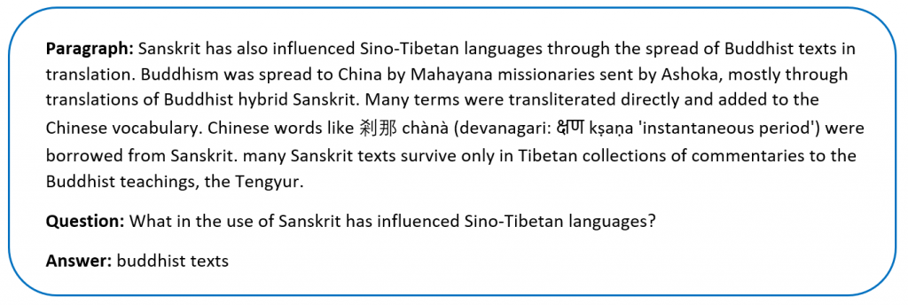
Rajpurkar, et al addressed the data issue by creating the SQuAD dataset in 2016 [11]. SQuAD uses articles sourced from Wikipedia and has more than 100,000 questions. The labelled data was obtained by crowdsourcing on Amazon Mechanical Turk – three human responses were taken for each answer and the official evaluation takes the maximum F1 and EM scores for each one.
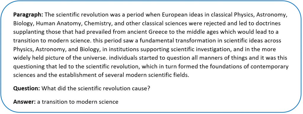
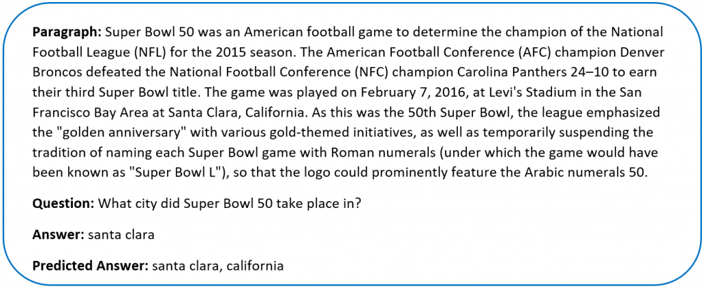
Sample SQuAD dataSince the release of SQuAD new research has pushed the boundaries of machine comprehension systems. Most of these use some form of Attention Mechanism [6][12][13] which tell the decoder layer to “attend” to specific parts of the source sentence at each step. Attention mechanisms address the problem of trying to encode the entire sequence into a final hidden state.
Formally we can define the task as follows – given a context paragraph c, a question q we need to predict the answer span by predicting (astart,aend) which are start and end indices of the context text where the answer lies.
For this project I implemented the Bidirectional Attention Flow model [6] – a hierarchical multi-stage model that has performed very well on the SQuAD dataset. I trained my own character vectors [15][16], and used pretrained Glove embeddings [14] for the word vectors. My final submission was a single model – ensemble models would typically yield better results but the complexity of my model meant longer training times.
Related Work
Since its introduction in June 2016, the SQuAD dataset has seen lots of research teams working on the challenge. There is a leaderboard maintained at https://rajpurkar.github.io/SQuAD-explorer/. Submissions since Jan 2018 have beaten human accuracy on one of the metrics (Microsoft Research, Alibaba and Google Brain are on this list at the time of writing this paper). Most of these models use some form of attention mechanism and ensemble multiple models.
For example, the R-Net by Microsoft Research [12] is a high performing SQuAD model. They use word and character embeddings along with Self-Matching attention. The Dynamic Coattention Network [13], another high performing SQuAD model uses coattention.
Approach
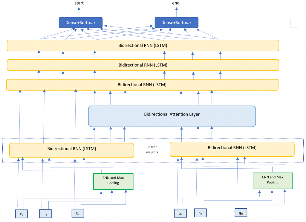
My model architecture is very closely based on the BiDAF model [6]. I implemented the following layers
- Embedding layer – Maps words to high dimensional vectors. The embedding layer is applied separately to both the context and question text. I used two methods
- Word embeddings – Maps each word to pretrained vectors. I used 300 dimensional GloVE vectors.
- Character embeddings – Maps each word to character embedding and run them through multiple layers of Convolutions and Max Pooling layers. I trained my own character embeddings due to challenges with the dataset.
- RNN Encoder layer – Takes the context and question embeddings and runs each one through a Bi-Directional RNN (LSTM). The Bi-RNNs share weights in order to enrich the context-question relationship.
- Attention Layer – Calculates the BiDirectional attention flow (Context to Query attention and Query to Context attention). We concatenate this with the context embeddings.
- Modeling Layer – Runs the attention and context layers through multiple layers of Bi-Directional RNNs (LSTMs)
- Output layer – Runs the output of the Modeling Layer through two fully connected layers to calculate the start and end indices of the answer span.
Dataset
The dataset for this project was SQuAD – a reading comprehension dataset. SQuAD uses articles sourced from Wikipedia and has more than 100,000 questions. Our task is to find the answer span within the paragraph text that answers the questions.
The sentences (all converted to lowercase) are tokenized into words using nltk. The words are then converted into high dimensional vector embeddings using Glove. The characters for each word are also converted into character embeddings and then run through a series of convolutions neural network and max pooling layers. I ran some analysis on the word and character counts in the dataset to better understand what model parameters to use.
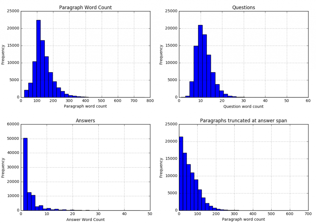 We can see that
| 99.8 percent of paragraphs are under 400 words |
| 99.9 percent of questions are under 30 words |
| 99 percent of answers are under 20 words (97.6 under 15 words) |
| 99.9 percent of answer spans lie within first 300 paragraph words |
We can use these statistics to adjust our model parameters (described in the next section).
For the character level encodings, I did an analysis of the character vocabulary in the training text. We had 1,258 unique characters. Since we are using Wikipedia for our training set, many articles contain foreign characters.
Further analysis suggested that these special characters don’t really affect the meaning of a sentence for our task, and that the answer span contained 67 unique characters. I therefore selected these 67 as my character vocabulary and replaced all the others with a special REPLACEMENT TOKEN.
Instead of using one-hot embeddings for character vectors, I trained my own character vectors on a subset of Wikipedia. I ran the word2vec algorithm at a character level to get char2vec 50 dimensional character embeddings. A t-SNE plot of the embeddings shows us results similar to word2vec.
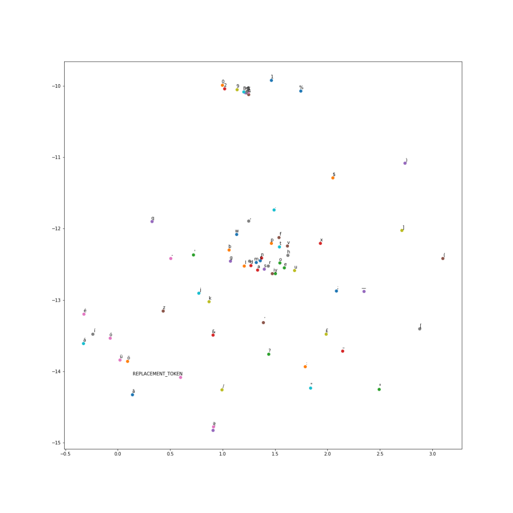 I used these trained character vectors for my character embeddings. The maximum length of a paragraph word was 37 characters, and 30 characters for a question word. Since we are using max pooling, I used these as my character dimensions and padded with zero vectors for smaller words.
Model Configuration
I used the following parameters for my model. Some of these (context length, question length, etc.) were fixed based on the data analysis in the previous section. Others were set by trying different parameters to see which ones gave the best results.
| Parameter | Description | Value |
| context_len | Number of words in the paragraph input | 300 |
| question_len | Number of words in the question input | 30 |
| embedding_size | Dimension of GLoVE embeddings | 300 |
| context_char_len | Number of characters in each word for the paragraph input (zero padded) | 37 |
| question_char_len | Number of characters in each word for the question input (zero padded) | 30 |
| char_embed_size | Dimension of character embeddings | 50 |
| optimizer | Optimizer used | Adam |
| learning_rate | Learning Rate | 0.001 |
| dropout | Dropout (used one dropout rate across the network) | 0.15 |
| hidden_size | Size of hidden state vector in the Bi-Directional RNN layers | 200 |
| conv_channel_size | Number of channels in the Convolutional Neural Network | 128 |
Evaluation metric
Performance on SQuAD was measured via two metrics:
- ExactMatch (EM) – Binary measure of whether the system output matches the ground truth exactly.
- F1 – Harmonic mean of precision and recall.
Results
My model achieved the following results (I scored much higher on the Dev and Test leaderboards than on my Validation set)
| Dataset | F1 | EM |
| Train | 81.600 | 68.000 |
| Val | 69.820 | 54.930 |
| Dev | 75.509 | 65.497 |
| Test | 76.553 | 66.401 |
The original BiDAF paper had an F1 score of 77.323 and EM score of 67.947. My model scored a little lower, possibly because I am missing some details not mentioned in their paper, or I need to tweak my hyperparameters further. Also, my scores were lower running against my cross validation set vs the official competition leaderboard.
I tracked accuracy on the validation set as I added more complexity to my model. I found it interesting to understand how each additional element contributed to the overall score. Each row tracks the added complexity and scores related to adding that component.
| Model | F1 | EM |
| Baseline | 39.34 | 28.41 |
| BiDAF | 42.28 | 31.00 |
| Smart Span (adjust answer end location) | 44.61 | 31.13 |
| 1 Bi-directional RNN in Modeling Layer | 66.83 | 51.40 |
| 2 Bi-directional RNNs in Modeling Layer | 68.28 | 53.10 |
| 3 Bi-directional RNNs in Modeling Layer | 68.54 | 53.25 |
| Character CNN | 69.82 | 54.93 |
I also analyzed the questions where we scored zero on F1 and EM scores. The F1 score is more forgiving. We would have a non zero F1 if we predict even one word correctly vs any of the human responses. An analysis of questions that scored zero on the F1and EM metric were split by question type. The error rates are proportional to the distribution of the questions in the dataset.
| Question Type | Entire Dev Set (%) | F1=0 (%) | EM=0 (%) |
| what | 27.2 | 28.4 | 29.3 |
| is | 18.4 | 18.5 | 18.4 |
| did | 9.1 | 8.8 | 9.0 |
| was | 8.7 | 9.1 | 7.9 |
| do | 6.9 | 6.9 | 7.9 |
| how | 6.2 | 5.9 | 6.1 |
| who | 6.2 | 6.7 | 6.1 |
| are | 4.4 | 3.7 | 4.2 |
| which | 3.3 | 3.4 | 3.1 |
| where | 2.3 | 2.5 | 2.5 |
| when | 3.9 | 2.9 | 2.3 |
| name | 1.8 | 1.5 | 1.5 |
| why | 0.7 | 0.6 | 1.3 |
| would | 0.7 | 0.9 | 0.9 |
| whose | 0.2 | 0.2 | 0.2 |
However, there were some questions where the system was very close to the correct answer, or the correct answer was technically wrong

Conclusion
Attention mechanisms coupled with deep neural networks can achieve competitive results on Machine Comprehension. For this project I implemented the BiDirectional attention flow model. My model accuracy was very close to the original paper. In the modeling layer we discovered that deeper networks do increase accuracy, but at a steeper computational cost.
For future work I would like to explore an ensemble of models – using different deep learning layers and attention mechanisms. Looking at the leaderboard (https://rajpurkar.github.io/SQuAD-explorer/), most of the top performing models are ensembles.
Sentiment Analysis of movie reviews part 2 (Convolutional Neural Networks)
In a previous post I looked at sentiment analysis of movie reviews using a Deep Neural Network. That involved using pretrained vectors (GLOVE in our case) as a bag of words and fine tuning them for our task.
We will try a different approach to the same problem – using Convolutional Neural Networks (aka Deep Learning). We will take the idea from the image recognition blog and apply it to text classification. The idea is to
- Vectorize at a character level, using just the characters in our text. We don’t use any pretrained vectors for word embeddings.
- Apply multiple convolutional and max pooling layers to the data.
- Generate a final output layer with softmax
- We’re assuming the Convolutional Neural Network will automatically detect the relationship between characters (pooling them into words and further understanding the relationships between words).
Our input data is just vectorizing each character. We take all the unique characters in our data, and the maximum sentence length and transform our input data into maximum_sentence_length X character_count for each sentence. For sentences with less than the maximum_length, we pad the remaining rows with zeros.
I used 2 1-Dimensional convolutional layers with filter size=3, stride=1 and hidden size=64 and relu for the non-linear activation (see the Image Recognition blog for an explanation on this). I also added a pooling layer of size 3 after each convolution.
Finally, I used 2 fully connected layers of sizes 1024 and 256 dropout probability of 0.5 (that should help prevent over fitting. The final layer uses a softmax to generate the output probabilities and we the standard cross entropy function for the loss. The learning is optimized using the Adam optimizer.
Overall the results are very close to the deep neural network. We get 59.2% using CNNs vs 62%. I think the accuracy is the maximum information we can extract from this data. What’s interesting is we used 2 completely different approaches – pretrained word vectors in the Neural Network case, and character level vectors in this Deep Learning case and we got similar results.
Next post we will explore using LSTMs on the same problem.
Source code available on request.
Evaluation of Machine Learning Trading Strategies Using Recurrent Reinforcement Learning
A few months ago I did the Stanford CS221 course (Introduction to AI). The course was intense, covering a lot of advanced material. For the final project I worked with 2 teammates (Tesa Ho and Albert Lau) on evaluating Machine Learning Strategies using Recurrent Reinforcement Learning. This is our final project submission.
Introduction
There have been several studies that propose using Recurrent Reinforcement Learning to
design profitable trading systems over longer time horizons [see Moody , David and Molina ].
A common practice at trading shops today is to develop a Supervised Learning classification
algorithm to predict whether or not there will be a move of +/- X bps in the next t time period.
Depending on the trading strategy, the model selection may be based on maximizing the
Precision, Accuracy, a mixture of both i.e. F-score, or a measure of profit (i.e. Sharpe Ratio). In
the case of the latter, the parameters of the trading strategy must also be optimized which often
requires brute force.
The direct reinforcement approach, on the other hand, differs from dynamic programming and
reinforcement algorithms such as TD-learning and Q-learning, which attempt to estimate a value
function for the control problem. For finance in particular, the presence of large amounts noise
and non stationarity in the datasets can cause severe problems for the value function approach.
The RRL direct reinforcement framework enables a simpler problem representation, avoids
Bellman’s curse of dimensionality and offers compelling advantages in efficiency.
This project will apply the Recurrent Reinforcement Learning methodology to intraday trading on
the Hong Kong futures exchange specifically the Hang Seng futures. A gradient ascent of the
Sortino Ratio (or Downside Deviation Ratio) was used to calculate the optimized weights to
determine the trade signal. The results indicate that profitability is dependent on the maximum
position allowed (the variable μ). We also develop a trading strategy using the Reinforcement
Learning framework to adapt predictions from a Supervised Learning algorithm and compare
the results to the Recurrent Reinforcement Learning results.
Model and Approach
Our model is based on the work of Molina and Moody. We use Recurrent Reinforcement
Learning to maximize the Sharpe Ratio or Sortino Ratio for a financial asset (Hang Seng
Futures in our case) over a selected training period, then apply the optimized weight parameter
to a test period. The trades and profitability are saved and the process of training and testing is
repeated for all data.
This report is based on 5 minute open, high, low, close prices for the Hang Seng front-month
futures from November 1, 2016 to August 31, 2017. The close price was used as the price
array, px , and was the basis of the log normal returns, rt .
![\[r_t = ln \frac{p_t}{p_{t-1}}\]](http://rohitapte.com/wp-content/ql-cache/quicklatex.com-c7e4ef98fcb9b24325cf613a22f5e307_l3.png "Rendered by QuickLaTeX.com")
Other variables used in the model are:
M = the window size of returns used in the recurrent reinforcement learning
N = number of iterations for the RL algo
μ = max position size
δ = transaction costs in bps per trade
numTrainDays = the number of training days used
numTestDays = the number of test days used
The trader is assumed to take only long, neutral, or short positions with a maximum position of
magnitude mu. The position Ft is established or maintained at the end of each time interval t
and is reassessed at the end of period t+1. Where Moody used a trader function of:
![\[F_t=tanh(w^Tx_t) \in \{1,0,-1\}\]](http://rohitapte.com/wp-content/ql-cache/quicklatex.com-275275bb0378eb68c80ec9f42e2f177d_l3.png "Rendered by QuickLaTeX.com")
We opt to use a risk adjusted trader function of:
![\[F_t=tanh(w^Tx_t) \in \{-1,1\}\]](http://rohitapte.com/wp-content/ql-cache/quicklatex.com-c13ffee0de5387531e1421302a9f5e4b_l3.png "Rendered by QuickLaTeX.com")
where
![\[x_t=[1,t_{t-M},\dots,r_t,F_{t-1}]\]](http://rohitapte.com/wp-content/ql-cache/quicklatex.com-ad91ee89d1c7a090748d41d9624beb6c_l3.png "Rendered by QuickLaTeX.com")
The trade cost, δ , associated with each trade is assumed to occur on the closing price at the
end of each time period t. A non-zero trading cost in bps is used to account for slippage, bid
ask spread, and associated trading fees.
The trade return, Rt , is defined as the return obtained from trading:
![\[R_t=\mu (F_{t-1}r_t -\delta \vert F_t-F_{t-1} \vert)\]](http://rohitapte.com/wp-content/ql-cache/quicklatex.com-3005bdbbd120cd4cd375472b7a729511_l3.png "Rendered by QuickLaTeX.com")
where
μ = maximum number of shares per transaction
δ = transaction cost in bps
The reward function that is traditionally used to compare trading strategies is the Sharpe Ratio.
The Sharpe Ratio takes the average of the trade returns divided by the standard deviation of the
trade returns. This penalizes strategies with large variance in returns.
![\[Sharpe Ratio=\frac{Avg R_t}{Std R_t}\]](http://rohitapte.com/wp-content/ql-cache/quicklatex.com-ab82f16b93facc1dd1ceeb71abe7f84b_l3.png "Rendered by QuickLaTeX.com")
However, variance in positive returns is acceptable so the Sortino Ratio, or Downside Deviation
Ratio, is a much more accurate measure of a strategy. The Sortino Ratio penalizes large
variations in negative.
![\[Sortino Ratio=\frac{Avg R_t}{Std R_{t<0}}\]](http://rohitapte.com/wp-content/ql-cache/quicklatex.com-5e9cd3fb40f8d79136417385ee63b835_l3.png "Rendered by QuickLaTeX.com")
The reinforcement learning algorithm adjusts the parameters of the system to maximize the
expected reward function. It can also be expressed as a function of profit or wealth, U(WT) , or
in our case, a function of the sequence of trading returns, U(R1 , R2 , …, RT). Given the trading
system Ft(θ) , we can then adjust the parameters θ to maximize UT . The optimized variable is
θ , an array of weights applied to the log normal price returns r_t−M , …, rt .
![\[\theta = \{w_1,\dots,w_M \}\]](http://rohitapte.com/wp-content/ql-cache/quicklatex.com-892e3143a0171be91e5cd263cddf5c8f_l3.png "Rendered by QuickLaTeX.com")
The gradient with respect to θ is:
![\[\frac{d U_T(\theta)}{d \theta} =\sum_{t=1}^T \frac{d U_t}{dR_t} \{ \frac{dR_t}{dF_t} \frac{dF_1}{d \theta} + \frac{d R_t}{d F_{t-1}} \frac{dF_{t-1}}{d \theta} \} \]](http://rohitapte.com/wp-content/ql-cache/quicklatex.com-52d8d732746b1e2065c055bc1e40d0d5_l3.png "Rendered by QuickLaTeX.com")
where
![\[\frac{dR_t}{dF_t}=-1 \mu \delta sign(F_t-F_{t-1}) \]](http://rohitapte.com/wp-content/ql-cache/quicklatex.com-f2d282e640babf7f573e62075e14abdd_l3.png "Rendered by QuickLaTeX.com")
![\[\frac{dR_t}{dF_{t-1}}=\mu r_t + \mu \delta sign(F_t-F_{t-1}) \]](http://rohitapte.com/wp-content/ql-cache/quicklatex.com-f9f901c3d7ee2cfb877b9fa129a71171_l3.png "Rendered by QuickLaTeX.com")
![\[\frac{dF_t}{d \theta}=(1-tanh(x_t \cdot \theta)^2)(x_t+w_M \cdot dF_{t-1}) \]](http://rohitapte.com/wp-content/ql-cache/quicklatex.com-2f1722c11cd4f025dc64dcb11f262994_l3.png "Rendered by QuickLaTeX.com")
![\[\frac{dU_t}{dR_t}=\frac{(Avg R_t^2-Avg R_t)R_t}{\sqrt{\frac{T}{T-1}} (Avg R_t^2-Avg(R_t)^2)^1.5} \]](http://rohitapte.com/wp-content/ql-cache/quicklatex.com-8ed057ffb04f8050e648defec31b350c_l3.png "Rendered by QuickLaTeX.com")
We can then maximize the Sharpe Ratio using Gradient Ascent or Stochastic Gradient Ascent to find the optimal weights for θ .
![\[\theta_t=\theta_{t-1} + \eta \frac{dU_r}{d \theta} \]](http://rohitapte.com/wp-content/ql-cache/quicklatex.com-0882f879d5009ba24761de49eb0b3c83_l3.png "Rendered by QuickLaTeX.com")
where
η = learning rate
Training and Testing Procedure
The overall algorithm utilized a rolling training and test period of 30 and 10 days.
- Training period 1-30 days, test period 30-40 days
- Run recurrent learning algorithm to maximize the Sortino Ratio by optimizing θ over the training period
- Apply the optimized θ to the test period and evaluate the trades and pnl
- Update the training period to 10-40 days, test period 40-50 days and repeat the process
Overall analysis was run over all the test periods with the positions and trades priced at the closing price for each time period, t. Cumulative pnl was used to evaluate the trading strategies rather than than returns since geometric cumulative returns were skewed by negative and close to zero return periods.
Evaluation and Error Analysis
For the base case we have extracted features using the market data (order book depth, cancellations, trades, etc.) and run a random forest algorithm to classify +/- 10 point moves in the future over 60 second horizons. Probabilities were generated for -1, 0, +1 classes and the largest probability determined the predicted class. The predicted signal of -1, 0, +1 was then passed to the recurrent reinforcement algorithm to determine what the risk adjusted pnl would be.
For the oracle, we pass the actual target signals to the recurrent reinforcement learning algorithm to see what the maximum trading pnl would be.
We want to see if the recurrent reinforcement learning algorithm can generate better results.
We will additionally explore if we can use LSTMs to predict the next price and see if they perform better than our base case. We will also explore adding the predicted log return into our Reinforcement learning model as an additional parameter to compare results.
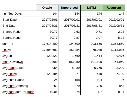
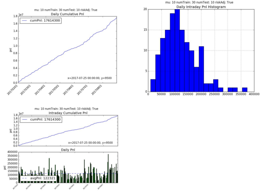
1. Oracle
The Oracle cumulative pnl over a 144 day test period is 17.6mm hkd. The average daily pnl is 122,321 hkd per day. The annualized Sharpe and Sortino ratio is 30.77 with an average of 25 trades a day.
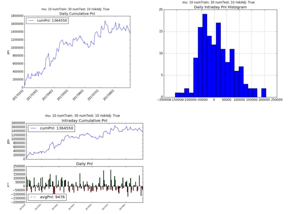
2. Recurrent Reinforcement Learning
The recurrent reinforcement learning cumulative pnl is 1.35 mm hkd with an average daily pnl is 9,476 hkd per day. The annualized Sharpe Ratio is 2.28 and Sortino Ratio is 5.08. The average number of trades per day is 106 with 8 contracts per trade.
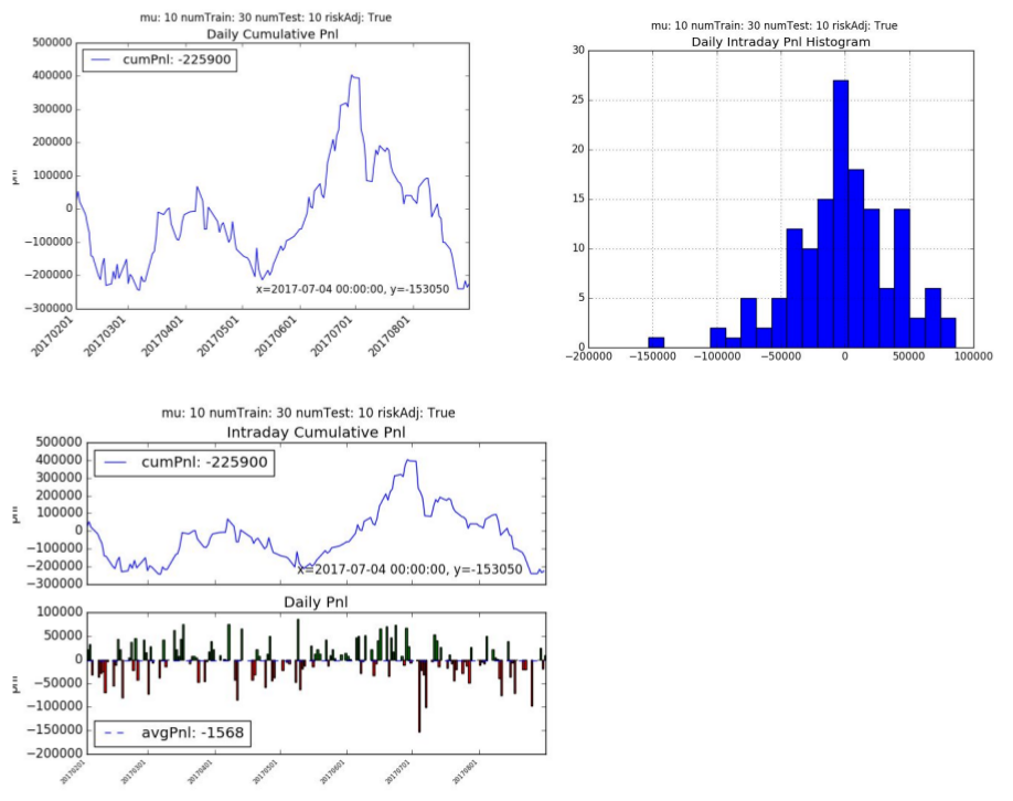
3. Supervised Learning
The supervised learning cumulative pnl is -226k hkd with an average daily pnl is -1568 hkd per day. The supervised learning model did not fair well with this trading strategy and had a Sharpe Ratio of -0.63 and Sortino Ratio of -0.87. The supervised learning algorithm traded much more frequently on average of 1,379 times a day with an average of 8.74 contracts per trade.
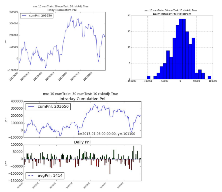
4. LSTM for Prediction
We also explored using LSTMs to predict +/- 10 point moves in the future over 60 second horizons. We used 30 consecutive price points (i.e. 30 minutes of trading data) to generate probabilities for (-1, 0 and +1).
One of the challenges we faced is the dataset is highly unbalanced, with approximately 94% of the cases being 0 (i.e. less than 10-tick move) and just 3% of the cases each being -1 (-10 tick move) or +1 (+10 tick move). Initially the LSTM was just calculating all items as 0 and getting a low error rate. We had to adjust our cross_entropy function to factor in the weights of the distribution which forced it try and classify the -1 and +1 more correctly.
We used a 1 layer LSTM with 64 hidden cells and a dropout of 0.2. Over the results were not great, but slightly better than the RandomForest.
The cumulative pnl is +203.65k hkd with an average daily pnl is +1414 hkd per day. The model had a Sharpe Ratio of 0.71 and Sortino Ratio of 1.07. The algorithm traded less frequently than supervised learning (on average of 104 times a day) but traded larger contracts. This makes sense since it’s classifying only a small percentage of the +/- 1 correctly.
5. Variable Sensitivity Analysis
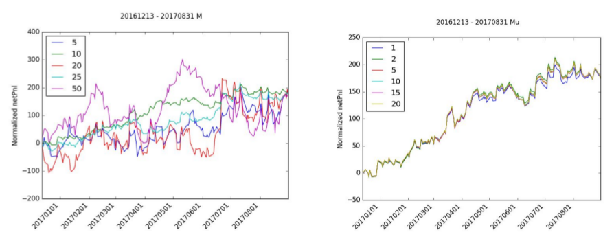
A sensitivity analysis was run to the following variables: M, μ, numTrainingDays, and N.
The selection of the right window period, M, is very important to the accumulation of netPnl. While almost all of the normalized netPnl ends at the same value, M=10 is the only value that has a stable increasing netPnl. M=20 and M=5 all have negative periods and M=50 has a significant amount of variance.
There is relatively little effect in normalized netPnl by adjusting mu. mu=1 has a slight drop in normalized pnl but still follows the same path as the other iterations.
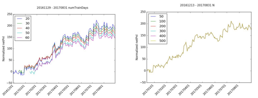
The number of training days has a limited effect on normalized netPnl since the shape of the pnl is roughly the same for each simulation. The starting point difference indicates that the starting month may or may not have been good months for trading. In particular, trading in January 2017 looked to be positive while the month of December was slightly negative.
Likewise, the number of iterations, N, has very little effect on normalized netPnl. The normalized netPnl is virtually identical for all levels of N.
Conclusions
Recurrent Reinforcement Learning (RRL) shows promise in trading financial markets. While it lacks behind the oracle, this has significant improvements over the current business standards with the use of supervised learning. While the RRL approach is sensitive to the choice the window size, it is plausible to note its limited business adoption to-date possibly for the below reasons.
- We have tested the algorithms on 144 days of data. We need to validate the test on a
larger set of historical data. - Trade price assumption is based on closing price and not next period open price. In live markets there would be some slippage from the time a signal was generated to when a trade was executed.
- We assume our execution costs are static. For larger trades, there would be more
slippage. We are also not making any assumptions about trading margin, both for new trades and drawdowns. In live trading these factors would affect position sizing and trades. - Incorporation of supervised prediction did not include positional risk adjustment
Gradient calculation for Sortino Ratio - Since 2008 markets have largely been in a low volatility regime. We need to test this algorithm under stressed markets to ensure it performs as expected and that drawdowns are reasonable.
- In the past 12 months the market has seen some strong directional themes. A simple quantitative momentum strategy would likely yield similar results.
- Further work has to be done to determine if RRL algorithms can outperform well established quantitative strategies.
Sentiment Analysis of movie reviews part 1 (Neural Network)
I’ve always been fascinated with Natural Language Processing and finally have a few tools under my belt to tackle this in a meaningful way. There is an old competition on Kaggle for sentiment analysis on movie reviews. The link to the competition can be found here.
As per the Kaggle website – the dataset consists of tab-separated files with phrases from Rotten Tomatoes. Each sentence has been parsed into many phrases by the Stanford parser. Our job is to learn on the test data and make a submission on the test data. This is what the data looks like.
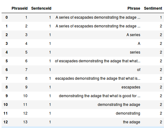
Each review (Sentiment in the above image) can take on values of 0 (negative), 1 (somewhat negative), 2 (neutral), 3 (somewhat positive) and 4 (positive). Our task is to predict the review based on the review text.
I decided to try a few techniques. This post will cover using a vanilla Neural Network but there is some work with the preprocessing of the data that actually gives decent results. In a future post I will explore more complex tools like LSTMs and GRUs.
Preprocessing the data is key here. As a first step we tokenized each sentence into words and vectorized the word using word embeddings. I used the Stanford GLOVE vectors. I assume word2vec would give similar results but GLOVE is supposedly superior since it captures more information of the relationships between words. Initially I ran my tests using the 50 dimensional vectors which gave about 60% accuracy on the test set and 57.7% on Kaggle. Each word then becomes a 50-dimensional vector.
For a sentence, we take the average of the word vectors as inputs to our Neural Network. This approach has 2 issues
- Some words don’t exist in the Glove database. We are ignoring them for now, but it may be useful to find some way to address this issue.
- Averaging the word embeddings means we fail to capture the position of the word in the sentence. That can have an impact on some reviews. For example if we had the following review
Great plot, would have been entertaining if not for the horrible acting and directing.
This would be a bad review but by averaging the word vectors we may be losing this information.
For the neural network I used 2 hidden layers with 1024 and 512 neurons. The final output goes through a softmax layer and we use the standard cross-entropy loss since this is a classification problem.
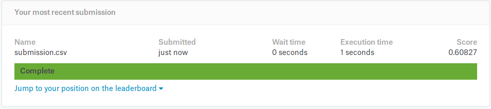
Overall the results are quite good. Using 100 dimensional GLOVE vectors, we get 62% accuracy on the test set and 60.8% on the Kaggle website.
Pre-trained vectors seem to be a good starting point to tackling NLP problems like this. The hyperparameter weight matrices will automatically tweak them for the task at hand.
Next steps are to explore larger embedding vectors and deeper neural networks to see if the accuracy improves further. Also play with regularization, dropout, and try different activation functions.
The next post will explore using more sophisticated techniques like LSTMs and GRUs.
Source code below (assuming you get the data from Kaggle)
|
1 2 3 4 5 6 7 8 9 10 11 12 13 14 15 16 17 18 19 20 21 22 23 24 25 26 27 28 29 30 31 32 33 34 35 36 37 38 39 40 41 42 43 44 45 46 47 48 49 50 51 52 53 54 55 56 57 58 59 60 61 62 63 64 |
import numpy as np import pandas as pd import numpy as np import csv #from nltk.tokenize import sent_tokenize,word_tokenize from nltk.tokenize import RegexpTokenizer from sklearn.preprocessing import LabelBinarizer from sklearn.model_selection import train_test_split glove_file='../glove/glove.6B.100d.txt' pretrained_vectors=pd.read_table(glove_file, sep=" ", index_col=0, header=None, quoting=csv.QUOTE_NONE) base_vector=pretrained_vectors.loc['this'].as_matrix() def vec(w): try: location=pretrained_vectors.loc[w] return location.as_matrix() except KeyError: return None def get_average_vector(review): numwords=0.0001 average=np.zeros(base_vector.shape) tokenizer = RegexpTokenizer(r'\w+') for word in tokenizer.tokenize(review): #sentences=sent_tokenize(review) #for sentence in sentences: # for word in word_tokenize(sentence): value=vec(word.lower()) if value is not None: average+=value numwords+=1 #else: # print("cant find "+word) average/=numwords return average.tolist() class SentimentDataObject(object): def __init__(self,test_ratio=0.1): self.df_train_input=pd.read_csv('/home/rohitapte/Documents/movie_sentiment/data/train.tsv',sep='\t') self.df_test_input=pd.read_csv('/home/rohitapte/Documents/movie_sentiment/data/test.tsv',sep='\t') self.df_train_input['Vectorized_review']=self.df_train_input['Phrase'].apply(lambda x:get_average_vector(x)) self.df_test_input['Vectorized_review'] = self.df_test_input['Phrase'].apply(lambda x: get_average_vector(x)) self.train_data=np.array(self.df_train_input['Vectorized_review'].tolist()) self.test_data=np.array(self.df_test_input['Vectorized_review'].tolist()) train_labels=self.df_train_input['Sentiment'].tolist() unique_labels=list(set(train_labels)) self.lb=LabelBinarizer() self.lb.fit(unique_labels) self.y_data=self.lb.transform(train_labels) self.X_train,self.X_cv,self.y_train,self.y_cv=train_test_split(self.train_data,self.y_data,test_size=test_ratio) def generate_one_epoch_for_neural(self,batch_size=100): num_batches=int(self.X_train.shape[0])//batch_size if batch_size*num_batches<self.X_train.shape[0]: num_batches+=1 perm=np.arange(self.X_train.shape[0]) np.random.shuffle(perm) self.X_train=self.X_train[perm] self.y_train=self.y_train[perm] for j in range(num_batches): batch_X=self.X_train[j*batch_size:(j+1)*batch_size] batch_y=self.y_train[j*batch_size:(j+1)*batch_size] yield batch_X,batch_y |
|
1 2 3 4 5 6 7 8 9 10 11 12 13 14 15 16 17 18 19 20 21 22 23 24 25 26 27 28 29 30 31 32 33 34 35 36 37 38 39 40 41 42 43 44 45 46 47 48 49 50 51 52 53 54 55 56 57 58 59 60 61 62 63 64 65 66 67 68 69 70 71 72 73 74 75 76 77 78 79 80 81 82 83 84 85 86 87 |
import tensorflow as tf import SentimentData #import numpy as np import pandas as pd sentimentData=SentimentData.SentimentDataObject() INPUT_VECTOR_SIZE=sentimentData.X_train.shape[1] HIDDEN_LAYER1_SIZE=1024 HIDDEN_LAYER2_SIZE=1024 OUTPUT_SIZE=sentimentData.y_train.shape[1] LEARNING_RATE=0.001 NUM_EPOCHS=100 BATCH_SIZE=10000 def truncated_normal_var(name, shape, dtype): return (tf.get_variable(name=name, shape=shape, dtype=dtype, initializer=tf.truncated_normal_initializer(stddev=0.05))) def zero_var(name, shape, dtype): return (tf.get_variable(name=name, shape=shape, dtype=dtype, initializer=tf.constant_initializer(0.0))) X=tf.placeholder(tf.float32,shape=[None,INPUT_VECTOR_SIZE],name='X') labels=tf.placeholder(tf.float32,shape=[None,OUTPUT_SIZE],name='labels') with tf.variable_scope('hidden_layer1') as scope: hidden_weight1=truncated_normal_var(name='hidden_weight1',shape=[INPUT_VECTOR_SIZE,HIDDEN_LAYER1_SIZE],dtype=tf.float32) hidden_bias1=zero_var(name='hidden_bias1',shape=[HIDDEN_LAYER1_SIZE],dtype=tf.float32) hidden_layer1=tf.nn.relu(tf.matmul(X,hidden_weight1)+hidden_bias1) with tf.variable_scope('hidden_layer2') as scope: hidden_weight2=truncated_normal_var(name='hidden_weight2',shape=[HIDDEN_LAYER1_SIZE,HIDDEN_LAYER2_SIZE],dtype=tf.float32) hidden_bias2=zero_var(name='hidden_bias2',shape=[HIDDEN_LAYER2_SIZE],dtype=tf.float32) hidden_layer2=tf.nn.relu(tf.matmul(hidden_layer1,hidden_weight2)+hidden_bias2) with tf.variable_scope('full_layer') as scope: full_weight1=truncated_normal_var(name='full_weight1',shape=[HIDDEN_LAYER2_SIZE,OUTPUT_SIZE],dtype=tf.float32) full_bias2 = zero_var(name='full_bias2', shape=[OUTPUT_SIZE], dtype=tf.float32) final_output=tf.matmul(hidden_layer2,full_weight1)+full_bias2 logits=tf.identity(final_output,name="logits") cost=tf.reduce_mean(tf.nn.softmax_cross_entropy_with_logits(logits=logits,labels=labels)) train_step=tf.train.AdamOptimizer(learning_rate=LEARNING_RATE).minimize(cost) correct_prediction=tf.equal(tf.argmax(final_output,1),tf.argmax(labels,1),name='correct_prediction') accuracy=tf.reduce_mean(tf.cast(correct_prediction,tf.float32),name='accuracy') init = tf.global_variables_initializer() sess = tf.Session() sess.run(init) test_data_feed = { X: sentimentData.X_cv, labels: sentimentData.y_cv, } for epoch in range(NUM_EPOCHS): for batch_X, batch_y in sentimentData.generate_one_epoch_for_neural(BATCH_SIZE): train_data_feed = { X: batch_X, labels: batch_y, } sess.run(train_step, feed_dict={X:batch_X,labels:batch_y,}) validation_accuracy=sess.run([accuracy], test_data_feed) print('validation_accuracy => '+str(validation_accuracy)) validation_accuracy=sess.run([accuracy], test_data_feed) print('Final validation_accuracy => ' +str(validation_accuracy)) #generate the submission file num_batches=int(sentimentData.test_data.shape[0])//BATCH_SIZE if BATCH_SIZE*num_batches<sentimentData.test_data.shape[0]: num_batches+=1 output=[] for j in range(num_batches): batch_X=sentimentData.test_data[j*BATCH_SIZE:(j + 1)*BATCH_SIZE] test_output=sess.run(tf.argmax(final_output,1),feed_dict={X:batch_X}) output.extend(test_output.tolist()) #print(len(output)) sentimentData.df_test_input['Classification']=pd.Series(output) #print(sentimentData.df_test_input.head()) #sentimentData.df_test_input['Sentiment']=sentimentData.df_test_input['Classification'].apply(lambda x:sentimentData.lb.inverse_transform(x)) sentimentData.df_test_input['Sentiment']=sentimentData.df_test_input['Classification'].apply(lambda x:x) #print(sentimentData.df_test_input.head()) submission=sentimentData.df_test_input[['PhraseId','Sentiment']] submission.to_csv('submission.csv',index=False) |