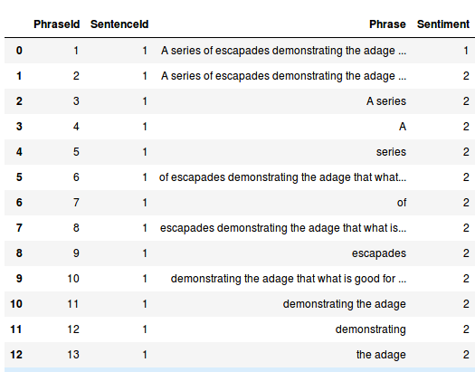
Love it or hate it Tesla as a company draws some very polarized opinions. Twitter is full of arguments both for and against the company. In this post we will see how to tackle this from an NLP perspective.
Disclaimer: This article is intended to purely show how to tackle this from an NLP perspective. I am currently short Tesla through stocks and options and any data and results presented here should not be interpreted as research or trading advice.
Fetching Twitter data
There are many libraries out there to fetch twitter data. The one I used was tweepy. I downloaded 25,000 of the most recent tweets and filtered for tweets in English. We were left with 18,171 tweets over a period of 9 days. Tweepy has a few configurable options. Unless you have a paid subscription you need to account for Rate Limiting. I also chose to filter out retweets and selected extended mode to get the full text of each tweet.
|
1 2 3 4 |
auth = tweepy.OAuthHandler(consumer_key, consumer_secret) auth.set_access_token(access_token, access_token_secret) api = tweepy.API(auth, wait_on_rate_limit=True) search_hashtag = tweepy.Cursor(api.search, q="TSLA -filter:retweets",tweet_mode='extended').items(25000) |
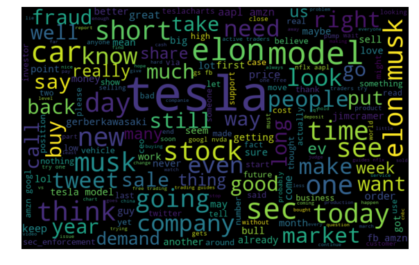
No NLP post is complete without a word cloud! We generate one on the twitter text removing stop words and punctuations. Its an interesting set of words – both positive and negative.
Sentiment Analysis
I found Vader (Valence Aware Dictionary and sEntiment Reasoner) to be a very good tool for Twitter sentiment analysis. It uses a lexicon and rule-based approach especially attuned to sentiments expressed in social media. Vader returns a score of 1 split across positive, neutral and and a compound score between -1 (extremely negative) and +1 (extremely positive). We use the compound score for our analysis. Here are the results for some sample tweets that it got correct.
|
1 2 3 4 5 6 7 8 9 10 |
If there was no fraud, there was no demand issue, no cash crunch, this is what would kill Tesla. Crafting artisan cars in the most expensive part of the world while competition is virtually fully automated already simply can't fly. Compound score: -0.9393 @GerberKawasaki Generational opportunity GERBER to add to TSLA longs. This might be the last chance to get in before she blows! Compound score: 0.6239 |
Vader gets plenty of classifications wrong. I guess the language for a stock is quite nuanced.
|
1 2 3 4 5 6 7 8 9 10 |
Today in "a company that is absolutely not experiencing a cash crunch". $TSLA Compound score: 0.0 Tesla (TSLA) Stock Ends the Week in Red. Are the Reasons Model Y or Musk Himself? #cryptocurrency #btcnews #altcoins #enigma #tothemoon #altcoins #pos Compound score: 0.0 Tesla (TSLA:NAS) and China Unicom (CHU:NYS) Upgraded Compound score: 0.0 |
One option is to train our own sentiment classifier if we can find a way to label data. But what about clustering tweets and analyzing sentiment by cluster? We may get a better understanding of which ones are classified correctly that way.
To cluster tweets we need to vectorize them so we can compute a distance metric. TFIDF works very well for this task. TFIDF consists of 2 components
Term Frequency – how often a word occurs in a document
Inverse Document Frequency – how much information the word provides (whether its common or rare across all documents).
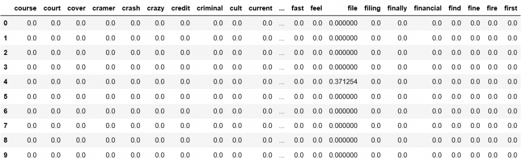
Before applying TFIDF we need to tokenize our words. I used NLTK’s TweetTokenizer which preserves mentions and $ tags, and lemmatized the words to collapse similar meaning words (we could also try stemming). I also removed all http links in tweets since we cant analyze them algorithmically. Finally I added punctuations to the stop words that TFIDF will ignore. I ran TFIDF using 1000 features. This is a parameter that we can experiment with and tune. This is what a sample subset of resultant matrix looks like.
We finally have a matrix we can use to run KMeans. Determining the number of clusters is a frequently encountered problem in clustering, different from the process of actually clustering the data. I used the Elbow Method to fine tune this parameter – essentially we try a range of clusters and plot the SSE (Sum of Squared Errors). SSE tends to 0 as we increase the cluster count. Plotting the SSE against number of errors tends to have the shape of an arm with the “elbow” suggesting at what value we start to see diminishing reduction in SSE. We pick the number of clusters to be at the elbow point.
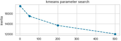
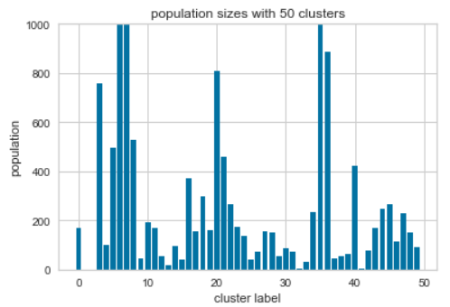
I decided to use 50 clusters since that’s where the elbow is. Its worth looking at a distribution of tweets for each cluster center and the most important features for clusters with a high population.
|
1 2 3 |
Cluster 6: ’ @elonmusk tesla elon ‘ musk stock #tesla sec time let going think today @tesla Cluster 7: @elonmusk #tesla @tesla stock time today would going cars short car company see day get Cluster 36: musk elon sec tesla ceo judge tweets contempt settlement via cramer going tesla's get |
Finally, to visualize the clusters we first use TSNE to reduce the TFIDF feature matrix to 2 dimensions, and then plot them using Bokeh. Bokeh lets us look at data when we hover over points to see how the clustering is working with text.
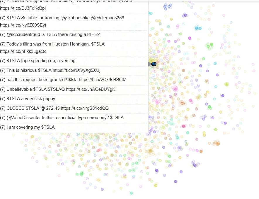
Analyzing the tweets and clusters I realized there is a lot of SPAM in twitter. For cleaner analysis its worth researching how to remove these tweets.
As usual, code is available on my Github.