Evaluation of Machine Learning Trading Strategies Using Recurrent Reinforcement Learning

A few months ago I did the Stanford CS221 course (Introduction to AI). The course was intense, covering a lot of advanced material. For the final project I worked with 2 teammates (Tesa Ho and Albert Lau) on evaluating Machine Learning Strategies using Recurrent Reinforcement Learning. This is our final project submission.

Introduction

There have been several studies that propose using Recurrent Reinforcement Learning to
design profitable trading systems over longer time horizons [see Moody , David and Molina ].
A common practice at trading shops today is to develop a Supervised Learning classification
algorithm to predict whether or not there will be a move of +/- X bps in the next t time period.
Depending on the trading strategy, the model selection may be based on maximizing the
Precision, Accuracy, a mixture of both i.e. F-score, or a measure of profit (i.e. Sharpe Ratio). In
the case of the latter, the parameters of the trading strategy must also be optimized which often
requires brute force.
The direct reinforcement approach, on the other hand, differs from dynamic programming and
reinforcement algorithms such as TD-learning and Q-learning, which attempt to estimate a value
function for the control problem. For finance in particular, the presence of large amounts noise
and non stationarity in the datasets can cause severe problems for the value function approach.
The RRL direct reinforcement framework enables a simpler problem representation, avoids
Bellman’s curse of dimensionality and offers compelling advantages in efficiency.
This project will apply the Recurrent Reinforcement Learning methodology to intraday trading on
the Hong Kong futures exchange specifically the Hang Seng futures. A gradient ascent of the
Sortino Ratio (or Downside Deviation Ratio) was used to calculate the optimized weights to
determine the trade signal. The results indicate that profitability is dependent on the maximum
position allowed (the variable μ). We also develop a trading strategy using the Reinforcement
Learning framework to adapt predictions from a Supervised Learning algorithm and compare
the results to the Recurrent Reinforcement Learning results.

Model and Approach

Our model is based on the work of Molina and Moody. We use Recurrent Reinforcement
Learning to maximize the Sharpe Ratio or Sortino Ratio for a financial asset (Hang Seng
Futures in our case) over a selected training period, then apply the optimized weight parameter
to a test period. The trades and profitability are saved and the process of training and testing is
repeated for all data.
This report is based on 5 minute open, high, low, close prices for the Hang Seng front-month
futures from November 1, 2016 to August 31, 2017. The close price was used as the price
array, p_x , and was the basis of the log normal returns, r_t .

$r_t = ln \frac{p_t}{p_{t-1}}$

Other variables used in the model are:
M = the window size of returns used in the recurrent reinforcement learning
N = number of iterations for the RL algo
μ = max position size
δ = transaction costs in bps per trade
numTrainDays = the number of training days used
numTestDays = the number of test days used
The trader is assumed to take only long, neutral, or short positions with a maximum position of
magnitude mu. The position F_t is established or maintained at the end of each time interval t
and is reassessed at the end of period t+1. Where Moody used a trader function of:

$F_t=tanh(w^Tx_t) \in \{1,0,-1\}$

We opt to use a risk adjusted trader function of:

$F_t=tanh(w^Tx_t) \in \{-1,1\}$

where

$x_t=[1,t_{t-M},\dots,r_t,F_{t-1}]$

The trade cost, δ , associated with each trade is assumed to occur on the closing price at the
end of each time period t. A non-zero trading cost in bps is used to account for slippage, bid
ask spread, and associated trading fees.
The trade return, R_t , is defined as the return obtained from trading:

$R_t=\mu (F_{t-1}r_t -\delta \vert F_t-F_{t-1} \vert)$

where
μ = maximum number of shares per transaction
δ = transaction cost in bps
The reward function that is traditionally used to compare trading strategies is the Sharpe Ratio.
The Sharpe Ratio takes the average of the trade returns divided by the standard deviation of the
trade returns. This penalizes strategies with large variance in returns.

$Sharpe Ratio=\frac{Avg R_t}{Std R_t}$

However, variance in positive returns is acceptable so the Sortino Ratio, or Downside Deviation
Ratio, is a much more accurate measure of a strategy. The Sortino Ratio penalizes large
variations in negative.

$Sortino Ratio=\frac{Avg R_t}{Std R_{t<0}}$

The reinforcement learning algorithm adjusts the parameters of the system to maximize the
expected reward function. It can also be expressed as a function of profit or wealth, U(W_T) , or
in our case, a function of the sequence of trading returns, U(R₁ , R₂ , …, R_T). Given the trading
system F_t(θ) , we can then adjust the parameters θ to maximize U_T . The optimized variable is
θ , an array of weights applied to the log normal price returns r__t−M , …, r_t .

$\theta = \{w_1,\dots,w_M \}$

The gradient with respect to θ is:

$\frac{d U_T(\theta)}{d \theta} =\sum_{t=1}^T \frac{d U_t}{dR_t} \{ \frac{dR_t}{dF_t} \frac{dF_1}{d \theta} + \frac{d R_t}{d F_{t-1}} \frac{dF_{t-1}}{d \theta} \}$

where

$\frac{dR_t}{dF_t}=-1 \mu \delta sign(F_t-F_{t-1})$

$\frac{dR_t}{dF_{t-1}}=\mu r_t + \mu \delta sign(F_t-F_{t-1})$

$\frac{dF_t}{d \theta}=(1-tanh(x_t \cdot \theta)^2)(x_t+w_M \cdot dF_{t-1})$

$\frac{dU_t}{dR_t}=\frac{(Avg R_t^2-Avg R_t)R_t}{\sqrt{\frac{T}{T-1}} (Avg R_t^2-Avg(R_t)^2)^1.5}$

We can then maximize the Sharpe Ratio using Gradient Ascent or Stochastic Gradient Ascent to find the optimal weights for θ .

$\theta_t=\theta_{t-1} + \eta \frac{dU_r}{d \theta}$

where
η = learning rate

Training and Testing Procedure

The overall algorithm utilized a rolling training and test period of 30 and 10 days.

Training period 1-30 days, test period 30-40 days
Run recurrent learning algorithm to maximize the Sortino Ratio by optimizing θ over the training period
Apply the optimized θ to the test period and evaluate the trades and pnl
Update the training period to 10-40 days, test period 40-50 days and repeat the process

Overall analysis was run over all the test periods with the positions and trades priced at the closing price for each time period, t. Cumulative pnl was used to evaluate the trading strategies rather than than returns since geometric cumulative returns were skewed by negative and close to zero return periods.

Evaluation and Error Analysis

For the base case we have extracted features using the market data (order book depth, cancellations, trades, etc.) and run a random forest algorithm to classify +/- 10 point moves in the future over 60 second horizons. Probabilities were generated for -1, 0, +1 classes and the largest probability determined the predicted class. The predicted signal of -1, 0, +1 was then passed to the recurrent reinforcement algorithm to determine what the risk adjusted pnl would be.
For the oracle, we pass the actual target signals to the recurrent reinforcement learning algorithm to see what the maximum trading pnl would be.
We want to see if the recurrent reinforcement learning algorithm can generate better results.
We will additionally explore if we can use LSTMs to predict the next price and see if they perform better than our base case. We will also explore adding the predicted log return into our Reinforcement learning model as an additional parameter to compare results.

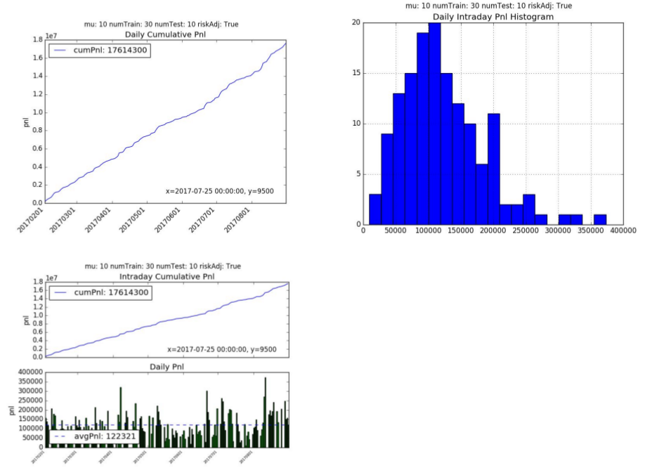
1. Oracle

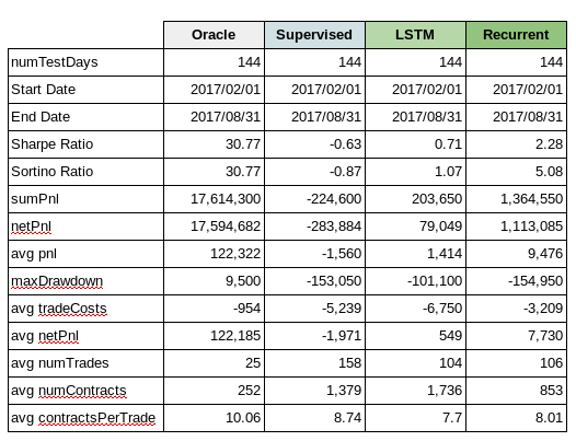
The Oracle cumulative pnl over a 144 day test period is 17.6mm hkd. The average daily pnl is 122,321 hkd per day. The annualized Sharpe and Sortino ratio is 30.77 with an average of 25 trades a day.

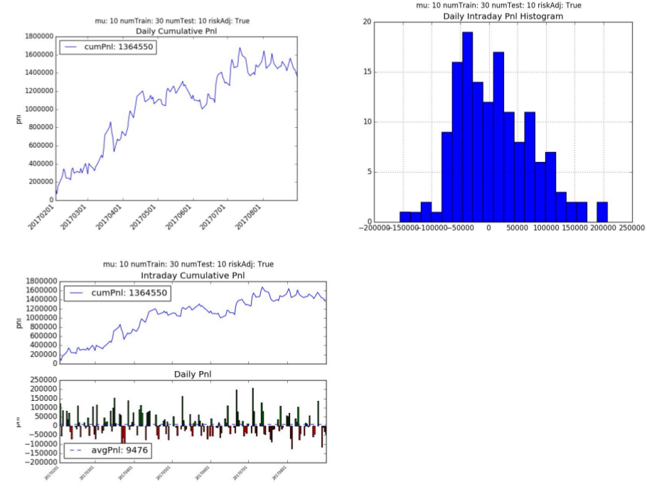
2. Recurrent Reinforcement Learning

The recurrent reinforcement learning cumulative pnl is 1.35 mm hkd with an average daily pnl is 9,476 hkd per day. The annualized Sharpe Ratio is 2.28 and Sortino Ratio is 5.08. The average number of trades per day is 106 with 8 contracts per trade.

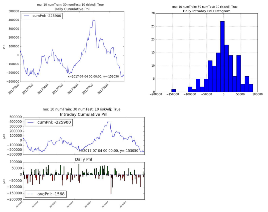
3. Supervised Learning

The supervised learning cumulative pnl is -226k hkd with an average daily pnl is -1568 hkd per day. The supervised learning model did not fair well with this trading strategy and had a Sharpe Ratio of -0.63 and Sortino Ratio of -0.87. The supervised learning algorithm traded much more frequently on average of 1,379 times a day with an average of 8.74 contracts per trade.

4. LSTM for Prediction

We also explored using LSTMs to predict +/- 10 point moves in the future over 60 second horizons. We used 30 consecutive price points (i.e. 30 minutes of trading data) to generate probabilities for (-1, 0 and +1).
One of the challenges we faced is the dataset is highly unbalanced, with approximately 94% of the cases being 0 (i.e. less than 10-tick move) and just 3% of the cases each being -1 (-10 tick move) or +1 (+10 tick move). Initially the LSTM was just calculating all items as 0 and getting a low error rate. We had to adjust our cross_entropy function to factor in the weights of the distribution which forced it try and classify the -1 and +1 more correctly.
We used a 1 layer LSTM with 64 hidden cells and a dropout of 0.2. Over the results were not great, but slightly better than the RandomForest.
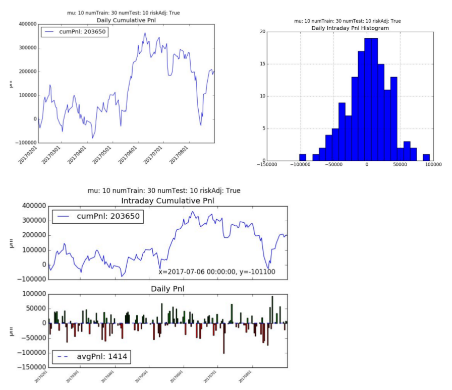
The cumulative pnl is +203.65k hkd with an average daily pnl is +1414 hkd per day. The model had a Sharpe Ratio of 0.71 and Sortino Ratio of 1.07. The algorithm traded less frequently than supervised learning (on average of 104 times a day) but traded larger contracts. This makes sense since it’s classifying only a small percentage of the +/- 1 correctly.

5. Variable Sensitivity Analysis

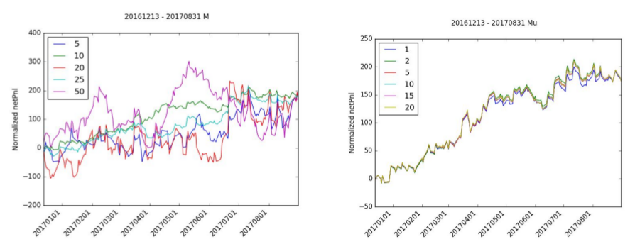
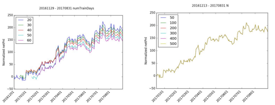
A sensitivity analysis was run to the following variables: M, μ, numTrainingDays, and N.

The selection of the right window period, M, is very important to the accumulation of netPnl. While almost all of the normalized netPnl ends at the same value, M=10 is the only value that has a stable increasing netPnl. M=20 and M=5 all have negative periods and M=50 has a significant amount of variance.

There is relatively little effect in normalized netPnl by adjusting mu. mu=1 has a slight drop in normalized pnl but still follows the same path as the other iterations.

The number of training days has a limited effect on normalized netPnl since the shape of the pnl is roughly the same for each simulation. The starting point difference indicates that the starting month may or may not have been good months for trading. In particular, trading in January 2017 looked to be positive while the month of December was slightly negative.

Likewise, the number of iterations, N, has very little effect on normalized netPnl. The normalized netPnl is virtually identical for all levels of N.

Conclusions

Recurrent Reinforcement Learning (RRL) shows promise in trading financial markets. While it lacks behind the oracle, this has significant improvements over the current business standards with the use of supervised learning. While the RRL approach is sensitive to the choice the window size, it is plausible to note its limited business adoption to-date possibly for the below reasons.

We have tested the algorithms on 144 days of data. We need to validate the test on a
larger set of historical data.
Trade price assumption is based on closing price and not next period open price. In live markets there would be some slippage from the time a signal was generated to when a trade was executed.
We assume our execution costs are static. For larger trades, there would be more
slippage. We are also not making any assumptions about trading margin, both for new trades and drawdowns. In live trading these factors would affect position sizing and trades.
Incorporation of supervised prediction did not include positional risk adjustment
Gradient calculation for Sortino Ratio
Since 2008 markets have largely been in a low volatility regime. We need to test this algorithm under stressed markets to ensure it performs as expected and that drawdowns are reasonable.
In the past 12 months the market has seen some strong directional themes. A simple quantitative momentum strategy would likely yield similar results.
Further work has to be done to determine if RRL algorithms can outperform well established quantitative strategies.